


 Abstract
 HTML
HTML Reference
 Related
 PDF
PDF


-
The quantum field theory (QFT) on the expanding portion of the de Sitter space-time [1] can be studied extensively, as the equations of the principal free fields, Klein-Gordon [2-8], Dirac [2, 9-18], and Proca [19, 20], can be solved analytically in various local charts. In the co-moving charts with Cartesian space coordinates, there are plane waves solutions that are eigenfunctions of the momentum operator, as in special relativity, but with more complicated time modulation functions that are generally linear combinations of Bessel functions dependent on the manner in which the frequencies are separated, thus fixing the vacuum. Unfortunately, in this geometry, one cannot use the energy operator to separate the frequencies as this does not commute with the momentum operator. Thus, the main task here is the criterion of separating the frequencies by defining the particle and antiparticle quantum modes [1].
The principal method used to date has primarily focused on the asymptotic states, which are somewhat similar to the usual Minkowskian particle or antiparticle states, as in the case of the adiabatic Bunch-Davies vacuum type [21] largely used in applications. The problem arising in this vacuum is that one cannot reach the rest limit for vanishing momentum, as this limit is undefined for the corresponding scalar mode functions or Dirac spinors. This problem has been considered sporadically by other authors, who have found similar results [2, 4, 7, 18].
Hence, we propose a method of separating the frequencies in rest frames, thus defining the rest frame vacuum (r.f.v.) of the massive Klein-Gordon [22], Dirac [23], and Proca [24] fields. The novelty of this approach is that the bosons can have either a tardyonic behavior or even a tachyonic one, if the mass is less than a given limit, which depends on the type of coupling (minimal or conformal). Fortunately, the tachyonic modes are eliminated in a natural manner as all their mode functions have null norms [22]. In contrast, the Dirac field of any non-vanishing mass survives in this vacuum [23]. In other respects, we must specify that the r.f.v. can be defined only for massive particles as the massless ones do not have rest frames. This is not an impediment because the massless fields of physical interest, namely the Maxwell and neutrino ones, have conformally covariant field equations for which the solutions in the co-moving de Sitter chart with conformal time can be drawn from special relativity [16, 25].
Technically speaking, to define the r.f.v., we introduced suitable phases depending on momentum to ensure the correct limits of the mode functions in rest frames [22-24]. Unfortunately, these phases are not sufficient to define the other important limit, namely the flat one, when the de Sitter Hubble constant tends to zero. In general, this limit is undefined because of singularities arising in the phases of the mode functions defined in the adiabatic vacuum. To remove these, a regularization procedure was applied by adding the convenient phase factors which, in general, depend on momentum [2, 4, 7, 18].
As this problem has not yet been considered for the recently defined r.f.v., the aim of this paper is to study the flat limits of the Klein-Gordon and Dirac fundamental solutions in this vacuum, deriving the regularized phases that guarantee that these limits are well-defined. In this manner, the rest and flat limits completely determine the form of the mode functions or spinors of the de Sitter QFT. This is important because there are quantities with expressions that are strongly dependent on the momentum-dependent phase factors, such as the one-particle energy (or Hamiltonian) operator [2, 6, 16]. We prove that the phase factors derived here determine the correct Minkowskian flat limit of this operator.
We specify that we recover previous results [2, 4, 7, 18] concerning the regularized phases, but the complete expressions of the scalar mode functions or Dirac spinors are presented here for the first time. Moreover, the approximations we obtain here are also new results that can be used in concrete calculations. However, the principal new result is that in the r.f.v., the flat limit is reached naturally, including for vanishing momenta, in contrast to the adiabatic vacuum in which the rest limit is undefined, forcing one to redefine the time modulation functions [7].
In the next section, we present the framework of our attempt to briefly review the theory of covariant fields on local-Minkowskian curved backgrounds, observing that these fields transform under isometries according to covariant representations (reps.) induced by the finite-dimensional reps. of the Lorentz group. In the second part of this section, the covariant reps. on the de Sitter space-time are considered focusing on their generators, which are the principal conserved observables of the quantum theory. The third section is devoted to the plane wave fundamental solutions of the Klein-Gordon and Dirac fields in the adiabatic and rest frame vacua, observing that the last vacuum naturally solves the rest limits. In the next section, we derive the flat limits of the aforementioned fields using a new uniform asymptotic expansion we propose here based on numerical arguments. This enables us to derive the regularized phases that ensure the flat limits of the fundamental solutions. Thus, we obtain, for the first time, complete expressions of the scalar mode functions and Dirac spinors in the r.f.v. as well as useful approximations of these quantities. Moreover, we show that in this approach, the flat limit of the one-particle energy operator is simply the corresponding operator of special relativity. Finally, we present our concluding remarks.
-
In local-Minkowskian space-time
$ (M,g) $ , we may introduce local charts$ \{t,\vec{x}\} $ for which the coordinates$ x^{\kappa} $ are labeled by the natural indices$ \kappa,\nu,... = 0,1,2,3 $ . The scalar, vector, and tensor fields can be defined locally on M using different classes of tensors that transform covariantly under diffeomorphisms and implicitly under isometries that are of physical interest, producing conserved quantities.The presence of the Dirac field requires orthogonal unholonomic (or local) frames in which the Dirac matrices make sense. These frames are defined by the tetrad vector fields
$ e_{\hat\alpha} = e_{\hat\alpha}^{\kappa}\partial_{\kappa} $ , while the co-frames are given by the dual 1-forms$ \omega^{\hat\alpha} = \hat e_{\kappa}^{\hat\alpha}dx^{\kappa} $ labeled by local indices$ \hat\kappa,\hat\nu,... = 0,1,2,3 $ . Given the tetrad components$ e_{\hat\alpha}^{\mu} $ and$ \hat e_{\mu}^{\hat\alpha} $ , one fixes the tetrad gauge. This can be changed at any time using the pseudo-orthogonal transformations$ \Lambda $ of the Lorentz group$ L_{+}^{\uparrow} $ which preserve the metric of M,$ g_{\kappa\nu} = \eta_{\hat\alpha\hat\beta}\hat e^{\hat\alpha}_{\kappa}\hat e^{\hat\beta}_{\nu} $ , because the Minkowski metric$ \eta = {\rm{diag}}(1, -1,-1,-1) $ is invariant under these transformations. Thus, we have to use frames$ \{x;e\} $ formed by a local chart and the local frames given by the tetrad fields. The task is now to construct a gauge-invariant theory independent of the gauge fixing. -
To obtain a gauge-invariant theory, we define the covariant fields
$ \psi_{(\rho)}:\, M\to {\cal{V}}_{(\rho)} $ , with values in the vector spaces$ {\cal{V}}_{(\rho)} $ carrying the finite-dimensional non-unitary rep.$ \rho $ of the group$ SL(2,{\mathbb{C}}) $ , which is the universal covering group of$ L_{+}^{\uparrow} $ [26, 27]. In the usual covariant parametrization, with the real parameters,$ \omega^{\hat\alpha \hat\beta} = -\omega^{\hat\beta\hat\alpha} $ , the transformations$ A(\omega) = \exp\left(-\frac{{\rm i}}{2}\omega^{\hat\alpha\hat\beta} S_{\hat\alpha\hat\beta}\right) \in SL(2,{\mathbb{C}}) $

(1) depend on the covariant basis-generators of the
$ sl(2,{{\mathbb{C}}}) $ Lie algebra,$ S_{\hat\alpha\hat\beta} $ . The transformations$\Lambda[A( \omega)] \in L_{+}^{\uparrow}$ associated to$ A(\omega) $ through the canonical homomorphism have the matrix elements$\Lambda^{\hat\mu\,\cdot}_{\cdot\,\hat\nu}[A(\omega)] = \delta^{\hat\mu}_{\hat\nu}+\omega^{\hat\mu\,\cdot}_{\cdot\,\hat\nu}+\cdots$ [28].The Lagrangian theory of the covariant field
$ \psi_{(\rho)} $ is gauge invariant if we replace the usual derivatives with the covariant ones,$ D_{\hat\alpha}^{(\rho)} = e_{\hat\alpha}^{\mu}D_{\mu}^{(\rho)} = \hat\partial_{\hat\alpha}+\frac{{\rm i}}{2}\, \rho(S^{\hat\beta\, \cdot} _{\cdot\, \hat\gamma})\,\hat\Gamma^{\hat\gamma}_{\hat\alpha \hat\beta}\,, $

(2) which depend on the connection coefficients in local frames (or spin connections),
$ \hat\Gamma^{\hat\sigma}_{\hat\mu \hat\nu} = e_{\hat\mu}^{\alpha} e_{\hat\nu}^{\beta}(\hat e_{\gamma}^{\hat\sigma} \Gamma^{\gamma}_{\alpha \beta} -\hat e^{\hat\sigma}_{\beta, \alpha})\,, $

(3) where
$ \Gamma^{\gamma}_{\alpha \beta} $ denote the Christoffel symbols.When
$ (M,g) $ has isometries$ x\to x' = \phi_{\frak g} (x) $ , these are, generally, non-linear reps.$ {\frak g}\to \phi_{\frak g} $ of the isometry group$ I(M) $ complying with the composition rule$ \phi_{\frak g}\circ \phi_{{\frak g}'} = \phi_{\frak{gg}'} $ ,$ \forall \frak{g,g}'\,\in I(M) $ . Denoting the identity function by$ id = \phi_{\frak e} $ , corresponding to the unit$ {\frak e}\in I(M) $ , we deduce$ \phi_{\frak g}^{-1} = \phi_{{\frak g}^{-1}} $ . In a given parametrization,$ {\frak g} = {\frak g}(\xi) $ (with$ {\frak e} = {\frak g}(0) $ ), the isometries$ x\to x' = \phi_{{\frak g}(\xi)}(x) = x+\xi^a k_a(x) +... $

(4) lay out the Killing vectors
$ k_a = \partial_{\xi_a}\phi_{{\frak g}(\xi)}|_{\xi = 0} $ associated to the parameters$ \xi^a $ ($ a,b,... = 1,2...N $ ).In general, the isometries may change the relative position of the local frames, thus affecting the physical interpretation. For this reason, we propose the theory of external symmetry [26], in which we introduce the combined transformations
$ (A_{\frak g},\phi_{\frak g}) $ that can correct the positions of the local frames. These transformations must preserve not only the metric but also the tetrad-gauge, transforming the 1-forms as$ \tilde\omega(x') = \Lambda[A_{\frak g}(x)]\tilde\omega(x) $ . Hereby, we deduce [26]$ \Lambda^{\hat\alpha\,\cdot}_{\cdot\,\hat\beta}[A_{\frak g}(x)] = \hat e_{\mu}^{\hat\alpha}[\phi_{\frak g}(x)]\frac{\partial \phi^{\mu}_{\frak g}(x)} {\partial x^{\nu}}\,e^{\nu}_{\hat\beta}(x)\,, $

(5) assuming, in addition, that
$ A_{{\frak g} = {\frak e}}(x) = 1\in SL(2,{\mathbb{C}}) $ . Then, the combined transformations$ (A_{\frak g},\phi_{\frak g}) $ preserve the gauge,$ ({A_{\frak g}},{\phi _{\frak g}}):\quad \begin{aligned} {e(x)}& \to &{e'(x')}& = &{e[{\phi _{\frak g}}(x)]{\mkern 1mu} ,}\\ {\hat e(x)}& \to &{\hat e'(x')}& = &{\hat e[{\phi _{\frak g}}(x)]{\mkern 1mu} ,}\end{aligned}$

(6) transforming the covariant fields according to the rule
$ (A_{\frak g},\phi_{\frak g}):\quad \psi_{(\rho)}(x)\to\psi_{(\rho)}'(x') = \rho[A_{\frak g}(x)]\psi_{(\rho)}(x)\,, $

(7) which defines the operator-valued rep.
$T^{(\rho)} \, : \, (A_{\frak g}, \phi_{\frak g}) \to T_{\frak g}^{(\rho)}$ , induced by$ \rho $ , the operators of which act as$ (T_{\frak g}^{(\rho)}\psi_{(\rho)})[\phi_{\frak g}(x)] = \rho[A_{\frak g}(x)]\psi_{(\rho)}(x)\,, $

(8) where
$ A_{\frak g}(x) $ is defined by Eq. (5).We have shown that the pairs
$ (A_{\xi},\phi_{\xi}) $ constitute a well-defined Lie group we refer to as the external symmetry group of$ (M,g) $ , denoted by$ S(M) $ , noting that this is just the universal covering group of$ I(M) $ [26]. Thus, we discuss the covariant reps. of the group$ S(M) $ induced by the reps.$ \rho $ of the group$ SL(2,,{\mathbb{C}}) $ . Note that, in the case of the integer spins, all the covariant fields are in fact vectors or tensors of different ranks transforming according to the established rules of general relativistic covariance [27].For each Killing vector
$ k_a $ defined by Eq. (4) there exists a corresponding generator of the rep. (8) that reads [26]$ \begin{aligned}[b]X^{(\rho)}_{a}& = {\rm i}{\partial_{\xi^a} T_{{\frak g}(\xi)}^{(\rho)}}_{|\xi = 0}\\ \;\;\;\;\;\;\;& = -{\rm i}k^{\mu}_{a}D_{\mu}^{(\rho)}+\frac{1}{2}\, k_{a\, \mu;\,\nu}\,e^{\mu}_{\hat\alpha}\,e^{\nu}_{\hat\beta}\, \rho(S^{\hat\alpha\hat\beta})\,,\end{aligned}$

(9) which is the generalization for any rep.
$ \rho $ of the formula given by Carter and McLenaghan for the Dirac field [29]. These operators are the principal conserved observables in the sense that they commute with the operator of the field equation resulting from the gauge-invariant Lagrangian theory [30].Another advantage of the Lagrangian theory is the possibility of introducing the relativistic scalar product
$ \langle \psi ,\psi'\rangle $ related to the natural$ U(1) $ symmetry of the free Lagrangian [1, 30]. We have shown that the relativistic scalar product is invariant under isometries$ \langle T_{\frak g}^{(\rho)}\psi, T_{\frak g}^{(\rho)}\psi'\rangle = \langle\psi,\psi'\rangle $ , while all the conserved observables (9) are self-adjoint with respect to this scalar product,$ \langle X_a^{(\rho)}\psi,\psi'\rangle = \langle\psi,X_a^{(\rho)}\psi'\rangle $ [30].In this framework, for any conserved operator X and field
$ \psi $ satisfying the field equation resulting from Lagrangian, we can construct the conserved quantity$ C[X] = \langle\psi,X\psi\rangle $ , which is interpreted as the expectation value at the level of relativistic quantum mechanics. After the second quantization, when the field$ \psi $ becomes a field operator, these quantities become the corresponding one-particle operators of the QFT [30],$ C[X]\; \; \to\; \; {\cal{X}} = :\langle\psi,X\psi\rangle: $

(10) calculated respecting the normal ordering of the field operators [31].
-
The
$ (1+3) $ -dimensional de Sitter space-time, denoted hereon by$ M,g $ , is the hyperboloid of radius$ \frac{1}{\omega} $ embedded in the$ (1+4) $ -dimensional pseudo-Euclidean space-time$ (M^5,\eta^5) $ of coordinates$ z^A $ (labeled by the indices$ A,\,B,... = 0,1,2,3,4 $ ) and metric$\eta^5 = {\rm{diag}}(1,-1, -1,-1,-1)$ [1]. The local charts of coordinates$ \{x\} $ can be easily introduced on$ (M,g) $ , giving the set of functions$ z^A(x) $ , which solve the hyperboloid equation$ \eta^5_{AB}z^A(x) z^B(x) = -\frac{1}{\omega^2}\,. $

(11) In this manner
$ (M,g) $ is defined as a homogeneous space of the pseudo-orthogonal group$ SO(1,4) $ , which is, at the same time, the gauge group of the metric$ \eta^{5} $ and the isometry group$ I(M) $ of the de Sitter space-time.The group of external symmetry,
$S(M) = {\rm{Spin}}(\eta^5) = Sp(2,2)$ , has the Lie algebra$ s(M) = sp(2,2)\sim so(1,4) $ , for which we use the covariant real parameters$ \xi^{AB} = -\xi^{BA} $ . Then, the orbital basis-generators of the natural rep. of the$ s(M) $ algebra (carried by the space of the scalar functions over$ M^{5} $ ) have the standard form$ L_{AB}^{5} = i\left[\eta_{AC}^5 z^{C}\partial_{B}- \eta_{BC}^5 z^{C} \partial_{A}\right] = -iK_{(AB)}^C\partial_C , $

(12) which allows us to derive the corresponding Killing vectors
$ k_{(AB)} $ by using the identities$ k_{(AB)\mu}dx^{\mu} = K_{(AB) C}dz^C $ . Thus, we obtain the components$ \xi_{(AB)} \; \; \to\; \; k_{(AB)\mu} = -z_A(x)\stackrel{\leftrightarrow}{\partial}_{\mu}z_B(x) , $

(13) with the notation
$ f\stackrel{\leftrightarrow}\partial g = f\partial g-g\partial f $ . These components will give rise to basis-generators of the covariant reps. according to Eq. (9).Exploiting the special coset structure of the de Sitter manifold,
$ M\sim SO(1,4)/ L_{+}^{\uparrow} $ , for the first time, Nachtmann constructed the covariant reps. of the group$ S(M) $ induced by the finite-dimensional reps. of the Lorentz group$ L_{+}^{\uparrow} $ [2]. We have shown that these are equivalent to our induced reps. presented above, thus proving the coherence of this theory in assuring the gauge invariance and giving rise to the conserved operators required [32].The hyperboloid equation is solved simply in the conformal chart
$ \{t_c,\vec{x}\} $ with the conformal time$ x^0 = t_c $ and Cartesian space coordinates$ x^i $ defined as$ \begin{aligned}[b]z^0(x) &= -\frac{1}{2\omega^2 t_c}\left[1-\omega^2({t_c}^2 - \vec{x}^2)\right]\,, \\ z^i(x) &= -\frac{1}{\omega t_c}x^i \,, \\ z^4(x) &= -\frac{1}{2\omega^2 t_c}\left[1+\omega^2({t_c}^2 - \vec{x}^2)\right]\,,\end{aligned} $

(14) giving the conformal flat line element
$ {\rm d}s^{2} = \eta^5_{AB}{\rm d}z^A(x){\rm d}z^B(x) = \frac{1}{\omega^2 {t_c}^2}\left({{\rm d}t_c}^{2}-{\rm d}\vec{ x}\cdot {\rm d}\vec{x}\right)\,. $

(15) In this chart, the de Sitter manifold M can be split into two parts: an expanding portion
$ M_+ $ and a collapsing one$ M_- $ , each with its own proper (or cosmic) time$ t\in(-\infty,\infty) $ defined as$ M_+ \; :\; \; -\infty<t_c = -\frac{1}{\omega}{\rm e}^{-\omega t}<0 \,, $

(16) $ M_- \; :\; \; \; \; \; \; \; 0<t_c = \frac{1}{\omega}{\rm e}^{\omega t}<\infty\,. $

(17) Physically speaking, the portion
$ M_+ $ is a convenient model of our actual universe called the de Sitter expanding universe. Moreover, if one considers physical processes on the whole de Sitter manifold, the effects on$ M_+ $ and$ M_- $ compensate each other, leading to null results [33]. For this reason, in the following, we restrict ourselves to the expanding portion$ M_+ $ , restricting$ t_c<0 $ such that in the chart$ \{t,\vec{x}\} $ of proper time, the line element takes the FLRW form$ {\rm d}s^2 = {\rm d}t^2-{\rm e}^{2\omega t} {\rm d}{\vec x}\cdot {\rm d}{\vec x}\,, $

(18) with the scale factor
$a(t) = {\rm e}^{\omega t}$ .The isometry group
$ I(M_+) $ of the expanding portion includes all the continuous transformations of the$ SO(1,4) $ group but only the discrete transformations preserving this portion. On this manifold, the basis-generators of the covariant reps. with a well-defined physical meaning are the energy H and momentum$ \vec{P} $ operators, which read [30, 34]$ H = \omega X_{(04)}^{(\rho)} = -i\omega(t_c\partial_{t_c}+x^i\partial_i) = i\partial_t-i\omega x^i\partial_i \,,\; \; \; \; $

(19) $ P^i = \omega(X_{(4i)}^{(\rho)}-X_{(0i)}^{(\rho)}) = -i\partial_i\,, $

(20) with no spin terms. In contrast, the components of angular momentum
$ {J}^{(\rho)}_i = \frac{1}{2}\,\epsilon_{ijk}X_{(jk)}^{(\rho)} $ and those of the dual momentum$ {Q}^{(\rho)}_i = \omega(X_{(4i)}^{(\rho)}+X_{(0i)}^{(\rho)}) $ have spin parts determined by the rep.$ \rho $ as in Ref. [34], but here, we do not use these operators.Respecting ad litteram the principles of the quantum theory, we assume that the quantum states of
$ M_+ $ are prepared or measured by a global apparatus represented by the operator algebra freely generated by the basis-generators of the covariant reps. This apparatus prepares quantum modes described by the fundamental solutions of the field equation which, in addition, are common eigenfunctions of a system of commuting conserved operators. Thus, the quantum modes are defined globally independent of the local coordinatization. Moreover, we require these fundamental solutions to form a basis (i.e., an orthonormal and complete system) with respect to the specific relativistic scalar product resulting from the Lagrangian theory [30]. The covariant quantum field can then be expanded in terms of fundamental solutions and particle and antiparticle operators. We have shown that these operators transform under isometries according to the unitary irreducible reps. of the$ Sp(2,2) $ group of the principal series exclusively [35, 36], for which the weights$ (p,q) $ depend on spin and rest energy [30, 34].Finally, we note that another attempt using de Sitter space-times considers only the unitary and irreducible linear reps. of the
$ Sp(2,2) $ group, transforming invariant fieldsdefined first on$ M^5 $ and then projected on M [37-40]. In this manner, one obtains a framework leading to different results, which cannot be related to those of the theory of covariant fields presented here. -
As mentioned, the fundamental solutions of the field equations can be determined as common eigenfunctions of a system of commuting operators, the eigenvalues of which play the role of integration constants with a precise physical meaning. When all the integration constants are determined in this manner, one can say that the system is complete. Unfortunately, the
$ so(1,4) $ algebra can offer us only incomplete systems, for example, the system$ \{P^1,P^2,P^3\} $ of plane waves. Thus, an integration constant remains arbitrary depending on the criterion of frequency separation we adopt, thus defining the vacuum.On
$ M_+ $ , we have so far the adiabatic Bunch-Davies vacuum type and the r.f.v. we introduced recently [22, 23]. Our principal objective is to study how the flat limit depends on the choice of these vacua, focusing on the Klein-Gordon and Dirac fields on$ M_+ $ . -
In the chart
$ \{t,\vec{x}\} $ , the scalar field$ \Phi : M_+\to {{\mathbb{C}}} $ of mass m, minimally coupled to the de Sitter gravity, satisfies the Klein-Gordon equation,$ \left( \partial_t^2-{\rm e}^{-2\omega t}\Delta +3\omega \partial_t+m^2\right)\Phi(x) = 0\,, $

(21) for which the general solutions can be expanded as
$ \begin{aligned}[b] \Phi(x) =& \Phi^{(+)}(x)+\Phi^{(-)}(x)\\ =& \int {\rm d}^3p \left[f_{\vec{p}}(x)a(\vec{p})+f_{\vec{p}}^*(x)b^{\dagger}(\vec{p})\right] \,, \end{aligned} $

(22) in terms of field operators
$ a(\vec{p}) $ and$ b(\vec{p}) $ , depending on the conserved momentum$ \vec{p} $ and plane wave fundamental solutions$ f_{\vec{p}} $ and$ f_{\vec{p}}^*(x) $ of positive and negative frequencies, respectively. These solutions are eigenfunctions of the momentum operators$ P^if_{\vec{p}} = p^i f_{\vec{p}} $ , which must be orthonormal in the momentum scale,$ \langle f_{\vec{p}},f_{\vec{p}'}\rangle_{KG} = -\langle f_{\vec{p}}^*,f_{\vec{ p}'}^*\rangle_{KG} = \delta^3(\vec{p}-\vec{p}')\,, $

(23) $ \langle f_{\vec{p}},f_{\vec{p}'}^*\rangle_{KG} = 0\,, $

(24) satisfying a completeness condition with respect to the relativistic scalar product [1]
$ \langle f,f'\rangle_{KG} = {\rm i}\int {\rm d}^3x\, a(t)^3\, f^*(x) \stackrel{\leftrightarrow}{\partial_{t}} f'(x)\,. $

(25) This gives the "squared norms"
$ \langle f,f\rangle_{KG} $ of the square integrable functions$ f\in {\cal{H}}\subset{\cal{K}} $ , which may have any sign when splitting the space of mode functions$ {\cal{K}} $ as$f \in \left\{ \begin{aligned} &{{{\cal{H}}_ + } \subset {{\cal{K}}_ + }}&{{\rm{if}}}&{{{\langle f,f\rangle }_{KG}} > 0{\mkern 1mu} ,}\\ &{{{\cal{H}}_0} \subset {{\cal{K}}_0}}&{{\rm{if}}}&{{{\langle f,f\rangle }_{KG}} = 0{\mkern 1mu} ,}\\ &{{{\cal{H}}_ - } \subset {{\cal{K}}_ - }}&{{\rm{if}}}&{{{\langle f,f\rangle }_{KG}} < 0{\mkern 1mu} .}\end{aligned} \right.$

(26) From a physical perspective, the mode functions of
$ {\cal{K}}_{\pm} $ are of positive/negative frequencies, whereas those of$ {\cal{K}}_0 $ do not have a physical meaning.The fundamental mode functions can be expressed as
$ f_{\vec{p}}(t,\vec{x}) = \frac{{\rm e}^{{\rm i} \vec{x}\cdot \vec{p}}}{[2\pi a(t)]^{\frac{3}{2}}}{\cal{F}}_p(t)\,, $

(27) in terms of the time modulation functions
$ {\cal{F}}_p: D_t\to {{\mathbb{C}}} $ , which depend on$ p = |\vec{p}| $ satisfying the equation$ \left[\frac{{\rm d}^2}{{\rm d}t^2}+\frac{p^2}{a(t)^2}+m^2-\frac{9}{4}\,\omega^2\right] {\cal{F}}_p(t) = 0\,, $

(28) and the normalization condition
$ \left({\cal{F}}_p, {\cal{F}}_p\right)\equiv i\,{\cal{F}}_p^*(t)\stackrel{\leftrightarrow}{\partial}_{t}{\cal{F}}_p(t) = 1\,, $

(29) which guarantees condition (23).
The general solution of Eq. (28) can be derived easily in the chart
$ \{t_c,\vec{x}\} $ obtaining [6, 22]$ {\cal{F}}_p(t_c) = \ c_1\phi_p(t_c) + c_2\phi_p^*(t_c)\,,\quad \phi_p(t_c) = \frac{1}{\sqrt{\pi\omega}}\,K_{\nu}({\rm i}pt_c)\,, $

(30) where
$ K_{\nu} $ is the modified Bessel function of the index$\nu= \left\{ {\begin{aligned}{\sqrt {\frac{9}{4} - {\mu ^2}} }\quad {{\rm{for}}}\quad {\mu < \frac{3}{2}}\\ {{\rm i}\kappa {\mkern 1mu} ,\kappa = \sqrt {{\mu ^2} - \frac{9}{4}} }\quad {{\rm{for}}}\quad {\mu > \frac{3}{2}}\end{aligned}} \right.{\mkern 1mu} , $

(31) where
$ \mu = \dfrac{m}{\omega} $ . The particular solution$ \phi_p(t_c) $ is normalized, i.e.,$ (\phi_p,\phi_p) = 1 $ , such that condition (29) is fulfilled only if we take$ \left|c_1\right|^2-\left|c_2\right|^2 = 1\,. $

(32) Thus, we remain with an undetermined integration constant that may be fixed by giving a criterion of frequency separation, thus setting the vacuum. Each pair of constants satisfying this condition determines a (generalized) basis
$ \{f_{\vec{p}}\,| \,\vec{p}\in {\mathbb{R}}^3_p\}\cup \{f_{\vec{p}}^*\,| \,\vec{p}\in {\mathbb{R}}^3_p\} $ of the physical space of mode functions$ {\cal{K}}_+\cup{\cal{K}}_- $ corresponding to the fixed vacuum.The most popular vacuum is the adiabatic Bunch-Davies type [21], with
$ c_1 = 1 $ and$ c_2 = 0 $ , which holds for any mass, regardless of the real or imaginary value of the index (31). Despite this advantage, here we face the problem of the rest limit, which cannot be defined as long as the functions$ K_{i\kappa} (ipt_c) $ have an ambiguous behavior,$ K_{{\rm i}\kappa} ({\rm i}pt_c)\propto \frac{1}{\Gamma\left(\dfrac{1}{2}-{\rm i}\kappa\right)}\left(\frac{{\rm i}pt_c}{2}\right)^{-{\rm i}\kappa}-\frac{1}{\Gamma\left(\dfrac{1}{2}+{\rm i}\kappa\right)}\left(\frac{{\rm i}pt_c}{2}\right)^{{\rm i}\kappa}\,, $

(33) for
$ p\to 0 $ , as it results from Eq. (A6). A possible solution is to redefine these functions by replacing${\rm i}\kappa\to {\rm i}\kappa \pm \epsilon$ to eliminate one of the above terms and introducing a convenient phase factor for the remaining one [2, 4, 7]. However, this procedure is palliative as this affects the physical meaning of the mass, which gains an imaginary part.To avoid these difficulties, we recently defined the r.f.v., separating the frequencies in the rest frames just as in special relativity [22]. Thus, we found that the rest energy,
$ M = \kappa\omega = \sqrt{m^2-\frac{9}{4}\omega^2}\,, \quad m>\frac{3}{2}\omega\,, $

(34) which plays the role of a dynamical mass, makes sense only for
$ \mu>\dfrac{3}{2} $ , as for$ \mu<\dfrac{3}{2} $ , the mode functions do not have a physical meaning, being of tachyonic type but with null norms. We have shown that in the tardyonic domain, this vacuum is stable, corresponding to the integration constants$ c_1 = -{\rm i}\left(\frac{p}{2\omega}\right)^{-{\rm i}\kappa}\frac{{\rm e}^{\pi\kappa}}{\sqrt{{\rm e}^{2\pi\kappa}-1}}\,, $

(35) $ c_2 = {\rm i}\left(\frac{p}{2\omega}\right)^{-{\rm i}\kappa}\frac{1}{\sqrt{{\rm e}^{2\pi\kappa}-1}}\,, $

(36) determining the time modulation functions of positive energy as [22]
$ {\cal{F}}_p(t_c) = \sqrt{\frac{\pi}{\omega}}\left(\frac{p}{2\omega}\right)^{-{\rm i}\kappa}\frac{I_{{\rm i}\kappa}({\rm i}pt_c)}{\sqrt{{\rm e}^{2\pi\kappa}-1}}\,. $

(37) We must specify that the above phase factor is introduced to ensure the correct rest limit
$ \mathop {\lim }\limits_{p \to 0} {\cal{F}}_p(t_c) = \frac{1}{\sqrt{2M}}\,{\rm e}^{-{\rm i} M t}\,, $

(38) calculated according to Eqs. (16) and (A6).
Finally, we must specify that the adiabatic and rest frame vacua are different from a physical perspective. First, they differ because in the adiabatic vacuum, the scalar particles may have any mass, whereas in the r.f.v. only the particles with
$ m>\frac{3}{2}\omega $ (in minimal coupling) can survive. Moreover, when this condition is accomplished, the basis of the adiabatic vacuum can be related to that of the r.f.v. through a non-trivial Bogolyubov transformation [1] for which the coefficients,$ \alpha\propto c_1 $ and$ \beta\propto c_2 $ , depend on the constants (35) and (36). -
The Dirac field transforms under isometries according to a rep. induced by the Dirac rep.
$ \rho_D = (\frac{1}{2},0)\oplus(0,\frac{1}{2}) $ of the$ SL(2,{{\mathbb{C}}}) $ , the generators of which depend on the point-independent Dirac$ \gamma $ -matrices,$ \gamma^{\hat\alpha} $ , labeled by local indices as$ \rho_D(S^{\hat\alpha\hat\beta}) = \frac{{\rm i}}{4}\left[\gamma^{\hat\alpha}, \gamma^{\hat\beta}\right]\,. $

(39) To express the covariant derivatives on
$ M_+ $ , we chose the diagonal tetrad-gauge defined as$ e_0 = \partial_t = \frac{1}{a(t_c)}\,\partial_{t_c}\,,\quad \; \; \; \; \omega^0 = {\rm d}t = a(t_c){\rm d}t_c\,, $

(40) $ e_i = \frac{1}{a(t)}\,\partial_i = \frac{1}{a(t_c)}\,\partial_i\,, \quad \omega^i = a(t){\rm d}x^i = a(t_c){\rm d}x^i\,,\; \; \; \; \; $

(41) to preserve the global
$ SO(3) $ symmetry, allowing us to systematically use the$ SO(3) $ vectors. In this tetrad-gauge, the covariant massive Dirac field$ \psi $ of mass m satisfies the equations$ (D_x-m) \psi (x) = 0 $ given by the Dirac operator$ D_x = {\rm i}\gamma^0\partial_{t}+ {\rm i} {\rm e}^{-\omega t}\gamma^i\partial_i +\frac{3{\rm i} \omega}{2} \gamma^{0}\,, $

(42) resulting from the Lagrangian theory [16, 30]. It is known that the last term of this operator can be removed at any time by substituting
$ \psi \to [a(t)]^{-\frac{3}{2}}\psi $ . Similar results can be written in the conformal chart.The general solution of the Dirac equation may be written as a mode integral,
$ \begin{aligned}[b]\psi({x}\,)& = \psi^{(+)}({x}\,)+\psi^{(-)}({x}\,)\\ \; \; \; \; & = \int {\rm d}^{3}p \sum\limits_{\sigma}[U_{\vec{p},\sigma}(x){\frak a}(\vec{p},\sigma) +V_{\vec{p},\sigma}(x){\frak b}^{\dagger}(\vec{p},\sigma)]\,,\end{aligned} $

(43) in terms of the fundamental spinors
$ U_{\vec{p},\sigma} $ and$ V_{\vec{p},\sigma} $ of positive and negative frequencies, respectively, which are plane wave solutions of the Dirac equation depending on the conserved momentum$ \vec{p} $ and an arbitrary polarization$ \sigma $ . These spinors satisfy the eigenvalue problems$ P^i U_{\vec{p},\sigma}(x) = p_iU_{\vec{p},\sigma}(x)\,, \quad P^i V_{\vec{p},\sigma}(x) = -p_iV_{\vec{p},\sigma}(x)\,, $

(44) and form an orthonormal basis related through the charge conjugation,
$ V_{\vec{p},\sigma}(t,\vec{x}) = U^c_{\vec{p},\sigma}(t,\vec{x}) = C\left[{U}_{\vec{p},\sigma}(t,\vec{x})\right]^* \,, \quad C = {\rm i}\gamma^2\,, $

(45) (see Appendix A); they also satisfy the orthogonality relations
$ \langle U_{\vec{p},\sigma}, U_{{\vec{p}\,}',\sigma'}\rangle_D = \langle V_{\vec{p},\sigma}, V_{{\vec{p}\,}',\sigma'}\rangle_D = \delta_{\sigma\sigma^{\prime}}\delta^{3}(\vec{p}-\vec{p}\,^{\prime})\; \; \; $

(46) $ \langle U_{\vec{p},\sigma}, V_{{\vec{p}\,}',\sigma'}\rangle _D = \langle V_{\vec{p},\sigma}, U_{{\vec{p}\,}',\sigma'}\rangle_D = 0\,, $

(47) with respect to the relativistic scalar product [16]
$ \langle \psi, \psi'\rangle_D = \int {\rm d}^{3}x\, a(t)^{3}\bar{\psi}(x)\gamma^{0}\psi(x)\,, $

(48) where
$ \bar{\psi} = \psi^+\gamma^0 $ is the Dirac adjoint of$ \psi $ . This basis is complete [16], defining the momentum rep. in which the particle$ ({\frak a},{\frak a}^{\dagger}) $ and antiparticle ($ {\frak b},{\frak b}^{\dagger}) $ operators satisfy the canonical anti-commutation relations [16].In the standard rep. of the Dirac matrices (with diagonal
$ \gamma^0 $ ), the general form of the fundamental spinors in momentum rep.,$ U_{\vec{p},\sigma}(t,\vec{x}\,) = \frac{{\rm e}^{{\rm i}\vec{p}\cdot\vec{x}}}{[2\pi a(t)]^{\frac{3}{2}}}\left( \begin{array}{c} u^+_p(t) \, \xi_{\sigma}\\ u^-_p(t) \, \dfrac{{p}^i{\sigma}_i}{p}\,\xi_{\sigma} \end{array}\right)\,, $

(49) $ V_{\vec{p},\sigma}(t,\vec{x}\,) = \frac{{\rm e}^{-{\rm i}\vec{p}\cdot\vec{x}}}{[2\pi a(t)]^{\frac{3}{2}}} \left( \begin{array}{c} v^+_p(t)\, \dfrac{{p}^i{\sigma}_i}{p}\,\eta_{\sigma}\\ v^-_p(t) \,\eta_{\sigma} \end{array}\right) \,, $

(50) is determined by the time modulation functions
$ u^{\pm}_p(t) $ and$ v^{\pm}_p(t) $ that depend only on t and$ p = |\vec{p}| $ . The Pauli spinors$ \xi_{\sigma} $ and$ \eta_{\sigma} = i\sigma_2 (\xi_{\sigma})^{*} $ have to be correctly normalized, i.e.,$ \xi^+_{\sigma}\xi_{\sigma'} = \eta^+_{\sigma}\eta_{\sigma'} = \delta_{\sigma\sigma'} $ , satisfying a natural completeness equation.The time modulation functions
$ u_p^{\pm}(t_c) $ and$ v_p^{\pm}(t_c) $ in the conformal chart satisfy the system$ \left[{\rm i}\partial_{t_c}\mp m\, a(t_c)\right]u_p^{\pm}(t_c) = {p}\,u_p^{\mp}(t_c)\,, $

(51) $ \left[{\rm i}\partial_{t_c} \mp m\, a(t_c)\right]v_p^{\pm}(t_c) = -{p}\,v_p^{\mp}(t_c)\,, $

(52) the prime integrals of which allow us to impose the charge conjugation symmetry (45) assuming that [23]
$ v_p^{\pm} = \left[u_p^{\mp}\right]^*\,, $

(53) and the normalization conditions
$ |u_p^+|^2+|u_p^-|^2 = |v_p^+|^2+|v_p^-|^2 = 1 \\ $

(54) which guarantee that Eqs. (46) and (47) are accomplished. As mentioned, these conditions cannot completely determine the solutions that have the general forms [23]
$ u^{+}_p(t_c) = \sqrt{-\frac{p t_c}{\pi}}\left[c_1 K_{\nu_{-}}\left({\rm i} p t_c\right)+c_2 K_{\nu_{-}}\left(-{\rm i} p t_c\right)\right]\,,\; \; \; \; $

(55) $ u^{-}_p(t_c) = \sqrt{-\frac{p t_c}{\pi}}\left[c_1 K_{\nu_{+}}\left({\rm i} p t_c\right)-c_2 K_{\nu_{+}}\left(-{\rm i} p t_c\right)\right]\,, $

(56) which are expressed in terms of modified Bessel functions
$ K_{\nu} $ of indices$\nu_{\pm} = \dfrac{1}{2}\pm {\rm i} \kappa$ , where now$ \kappa = \dfrac{m}{\omega} $ , and depend on the integration constants$ c_1 $ and$ c_2 $ , which must satisfy$ |c_1|^2+|c_2|^2 = 1\,, $

(57) to accomplish the normalization condition (54). The functions
$ v_p^{\pm} $ result from Eq. (53).Thus, we derive the general structure of the covariant Dirac field (43), for which the field operators
$ {\frak a}(\vec{p},\sigma) $ and$ {\frak b}(\vec{p},\sigma) $ transform according to the unitary irreducible reps. of the principal series$ (\dfrac{1}{2},\nu_{\pm}) $ , which are equivalent with the same Casimir invariants$ C_1 = m^2+\dfrac{3}{2}\omega^2 $ and$ C_2 = \dfrac{3}{4}\left(m^2+\dfrac{1}{4}\omega^2\right) $ [30, 34].To completely determine our solutions we must adopt the criterion of frequency separation. The adiabatic vacuum may be defined simply by choosing
$ c_1 = 1 $ and$ c_2 = 0 $ as in Refs. [2, 16]. The major problem of this vacuum is that in the momentum-spin rep., we cannot reach the rest frame limit even though the functions$ K_{\nu} $ now have defined limits for$ p\to 0 $ . This is because of the term$ \dfrac{\vec{p}\cdot\vec{\sigma}}{p} $ , for which the limit is undefined [23]. Moreover, if we force the limit vanishing this term by hand, we affect the normalization [16, 18].The solution is to adopt the r.f.v., imposing the conditions [23]
$ \mathop {\lim }\limits_{p \to 0} u_p^ - (t) = \mathop {\lim }\limits_{p \to 0} v_p^ + (t) = 0{\mkern 1mu} , $

(58) which remove the contribution of the aforementioned terms in rest frames. These conditions are accomplished only if we take
$ c_1 = \frac{{\rm e}^{\pi\kappa}p^{-{\rm i}\kappa}}{\sqrt{1+{\rm e}^{2\pi \kappa}}}\,, \quad c_2 = \frac{{\rm i}\,p^{-{\rm i}\kappa}}{\sqrt{1+{\rm e}^{2\pi \kappa}}}\,, $

(59) determining the definitive form of the modulation functions of positive frequencies as [23]
$ u_p^{\pm}(t_c) = \pm \frac{\sqrt{-\pi t_c}\, p^{\nu_-}}{\sqrt{1+{\rm e}^{2\pi\kappa}}}\, I_{\mp\nu_{\mp}}({\rm i}pt_c)\,. $

(60) The modulation functions of the negative frequencies have to be calculated according to Eq. (53). Thus, we obtain fundamental spinors for which the rest limits
$ \mathop {\lim }\limits_{\vec p \to 0} {U_{\vec p,\sigma }}(t,\vec x) = \frac{{{{\rm e}^{ -{\rm i}mt}}}}{{{{[2\pi a(t)]}^{\frac{3}{2}}}}}\left( {\begin{array}{*{20}{c}} {{\xi _\sigma }}\\ 0 \end{array}} \right){\mkern 1mu} , $

(61) $ \mathop {\lim }\limits_{\vec p \to 0} {V_{\vec p,\sigma }}(t,\vec x) = \frac{{{{\rm e}^{{\rm i}mt}}}}{{{{[2\pi a(t)]}^{\frac{3}{2}}}}}\left( {\begin{array}{*{20}{c}} 0\\ {{\eta _\sigma }} \end{array}} \right){\mkern 1mu} , $

(62) indicate that the rest energy of the Dirac field is m, as in special relativity.
In contrast to the Klein-Gordon field, the r.f.v. of the Dirac field holds for any mass, separating the frequencies just as in special relativity. Nevertheless, its relation with the adiabatic vacuum is similar to that in the scalar case because the basis of the adiabatic vacuum is related to that of the r.f.v. through a non-trivial Bogolyubov transformation, the coefficients of which are proportional to the constants (59).
-
The time modulation functions studied above depend on the variable
$ x = -p t_c = \frac{p}{\omega}{\rm e}^{-\omega t} $

(63) which in the rest limit, tends to
$ 0 $ but in the flat limit, when$ \omega \to 0 $ and$ -\omega t_c \to 1 $ , tends to infinity. Therefore, to analyze the behavior of the time modulation functions in the flat limit, we need to use a uniform expansion of the Bessel function$ J_{i\kappa+\lambda}(\kappa x) $ for large values of$ \kappa>0 $ , any$ x>0 $ , and$ \lambda = 0,\pm\frac{1}{2} $ . Unfortunately, we have a rigorous proof only for$ \lambda = 0 $ such that we are forced to generalize this case based on analytical and numerical arguments. -
We propose a generalization of the standard uniform asymptotic expansion (A8) to
$ J_{i\kappa+\lambda}(\kappa x) $ , observing that this is analytic in$ \kappa $ such that we can replace$ i\kappa \to i\kappa+\lambda $ without affecting the variable x or expressions containing it, such as$ \kappa x $ or$ \kappa\sqrt{1+x^2} $ . Therefore, we assume that the following approximation,$ \begin{aligned}[b]J_{i\kappa+\lambda}(\kappa x) \simeq {\cal{J}}(\kappa,\lambda, x) =& \frac{{\rm e}^{\frac{\pi\kappa}{2}-\frac{{\rm i}\pi\lambda}{2}}}{\sqrt{2\kappa\pi}}\\ \; \; \; \; \;& \times\frac{{\rm e}^{{\rm i} \kappa\sqrt{1+x^2}-\frac{{\rm i}\pi}{4}}}{ (1+x^2)^{\frac{1}{4}}} \left(\frac{1}{x}+\sqrt{1+\frac{1}{x^2}}\right)^{-{\rm i}\kappa-\lambda}\,,\end{aligned} $

(64) in which we neglected the terms of the order
$ {\cal{O}}(\kappa^{-1}) $ , holds even for non-vanishing values of$ \lambda\in {\mathbb{R}} $ . However, the crucial point is to verify whether this approximation is numerically satisfactory, comparing the functions J and$ {\cal{J}} $ .We start with the observation that, in our case, the variable (63) is positively defined without reaching the value
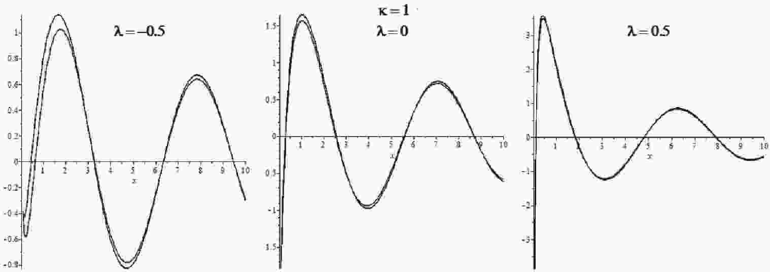
$ x = 0 $ if$ p\not = 0 $ , such that we can restrict our graphical study to the interval$ 0.1\leqslant x \leqslant 10 $ . Then, we may ask what it means by "large values of$ \kappa $ " plotting the functions J and$ {\cal{J}} $ on this interval. Thus, we see that their graphs tend to approach each other even for modest values of$ \kappa $ as in Fig. 1, where$ \kappa = 1 $ and$ \lambda = 0,\pm \frac{1}{2} $ . For larger values of$ \kappa $ (e.g.,$ \kappa>4 $ ), the graphs of these functions overlap such that we need to resort to the function
Figure 1. (color online) Functions
$\Re\,J_{i\kappa+\lambda}(\kappa x)$ (red) and$\Re\,{\cal{J}}(\kappa,\lambda, x)$ (blue) for$\kappa = 1$ and$\lambda = -\frac{1}{2},0, \frac{1}{2}$ .$ {\cal{E}}(\kappa,\lambda,x) = 1-\frac{{|{\cal{J}}|}(\kappa,\lambda,x)|}{|J_{i\kappa+\lambda}(\kappa x)|}\,, $

(65) to discern the errors of our approximation. In Fig. 2, we see how the errors diminish as
$ \kappa $ increases from$ 5 $ to$ 10 $ .
Figure 2. (color online) Function
${\cal{E}}(\kappa,\lambda, x)$ for$\kappa = 5$ (upper panels) and$\kappa = 10$ (lower panels).The conclusion is that our approximation is numerically satisfactory even for
$ \lambda \not = 0 $ . In practice, it is convenient to substitute$ \kappa x \to x $ to obtain the more homogeneous approximation$ J_{{\rm i}\kappa+\lambda}(x)\simeq\frac{{\rm e}^{\frac{\pi\kappa}{2}-\frac{{\rm i}\pi\lambda}{2}}}{\sqrt{2\pi}}\,\frac{{\rm e}^{{\rm i} \sqrt{\kappa^2+x^2}-\frac{{\rm i}\pi}{4}}}{ (\kappa^2+x^2)^{\frac{1}{4}}} \left(\frac{\kappa}{x}+\sqrt{1+\frac{\kappa^2}{x^2}}\right)^{-{\rm i}\kappa-\lambda}\,, $

(66) which is useful in investigating the flat limits of the scalar and spinor fields.
-
Let us briefly analyze the flat limits, for
$ \omega\to 0 $ , of the mode functions in the r.f.v. for$ \kappa>\frac{3}{2} $ , starting with rewriting the time modulation functions (37), according to Eq. (A7), as$ {\cal{F}}_p(t) = {\rm e}^{{\rm i}\delta_{KG}(p)}\left(\frac{p}{2\omega}\right)^{-{\rm i}\kappa}\sqrt{\frac{\pi}{\omega}}\frac{{\rm e}^{\frac{1}{2}\pi\kappa}}{\sqrt{{\rm e}^{2\pi\kappa}-1}}\,J_{{\rm i}\kappa}\left(\frac{p}{\omega}{\rm e}^{-\omega t}\right)\,. $

(67) Here, we introduce the auxiliary phase
$ \delta_{KG}(p) $ required for removing the pole in$ \omega = 0 $ of the general phase. Note that the second phase factor ensures the correct rest frame limit for$ p\to 0 $ [22]. The flat limit can be evaluated using the uniform expansion of this Bessel function (66) in which we substitute x as in Eq. (63). Then, according to Eq. (66), we may approximate$ {\cal{F}}_p(t_c)\simeq\rho(p,t){\rm e}^{{\rm i}\theta(p,t)}\,, $

(68) where
$ \rho(p,t) = \frac{1}{\sqrt{2}(M^2+p^2{\rm e}^{-2\omega t})^{\frac{1}{4}}}\frac{{\rm e}^{\pi\kappa}}{\sqrt{{\rm e}^{2\pi\kappa}-1}}\,, $

(69) $ \begin{aligned}[b]\theta(p,t) = &\delta_{KG}(p)-\frac{\pi}{4}-\frac{M}{\omega} \ln\left(\frac{1}{2\omega}\right)-Mt\\ &-\frac{M}{\omega}\ln\left(M+\sqrt{M^2 +p^2{\rm e}^{-2\omega t}}\right)\\ &+\frac{1}{\omega}\sqrt{M^2+p^2{\rm e}^{-2\omega t}}\,.\end{aligned}$

(70) Furthermore, we compute the series of
$ \theta(p,t) $ around$ \omega = 0 $ , where this function has a pole that can be removed by setting$ \delta_{KG}(p) = \frac{\pi}{4}+\frac{M}{\omega}\ln \frac{M+\sqrt{M^2+p^2}}{2\omega}-\frac{\sqrt{M^2+p^2}}{\omega}\,. $

(71) In this manner, we generate the phase factor
$ {\rm e}^{{\rm i}\delta_{KG}(p)} = {\rm e}^{\frac{{\rm i} \pi}{4}}\left(\frac{M+\sqrt{M^2+p^2}}{2\omega} \right)^{\frac{iM}{\omega}}{\rm e}^{-{\rm i}\frac{\sqrt{M^2+p^2}}{\omega}}\,, $

(72) without physical significance but necessary for deriving the convenient approximation that can be used in applications,
$ {\cal{F}}_p(t)\simeq\frac{{\rm e}^{\pi\kappa}}{\sqrt{{\rm e}^{2\pi\kappa}-1}}\frac{{\rm e}^{{\rm i}\theta_{KG}(p,t)}}{\sqrt{2}(M^2+p^2{\rm e}^{-2\omega t})^{\frac{1}{4}}}\,. $

(73) The regularized phase
$ \begin{aligned}[b] \theta_{KG}(p,t) =& -Mt -\frac{M}{\omega}\ln\left(\frac{M+\sqrt{M^2+p^2{\rm e}^{-2\omega t}}}{M+\sqrt{M^2+p^2}}\right)\\ \;\;\;\;\;\;\;\;\;\;\;\;\;&+\frac{1}{\omega}\left(\sqrt{M^2+p^2{\rm e}^{-2\omega t}}-\sqrt{M^2+p^2}\right)\,, \end{aligned}$

(74) is obtained by substituting into Eq. (70) the phase
$ \delta_{KG} $ defined by Eq. (71). For small values of$ \omega $ , we may use the Taylor series$ \begin{aligned}[b] \theta_{KG}(p,t) =& -\sqrt{M^2+p^2}\,t+\frac{\omega p^2 t^2}{2\sqrt{M^2+p^2}}\\ &-\frac{\omega^2 p^2(2M^2+p^2)t^3}{6(M^2+p^2)^\frac{3}{2}}+{\cal{O}}(\omega^3)\,, \end{aligned}$

(75) finding that in the flat limit, when
$ \lim_{\omega\to 0}M = m $ , and$ \mathop {\lim }\limits_{\omega \to 0} {\cal{F}}_p(t) = \frac{{\rm e}^{-{\rm i}E(p)t}}{\sqrt{2E(p)}}\,, \quad E(p) = \sqrt{m^2+p^2}\,, $

(76) we recover just the Minkowskian time modulation functions.
-
To analyze how the flat limit can be reached in the case of the Dirac field, it is convenient to rewrite the time modulation functions (60) in the chart
$ \{t,\vec{x}\} $ as$\begin{aligned}[b] u_p^{\pm}(t) =& \pm {\rm e}^{{\rm i}\delta_D(p)\pm \frac{{\rm i}\pi}{4}} p^{-{\rm i}\kappa}\\ \;\;\;\;\;\;\;\;\; &\times \frac{{\rm e}^{\frac{\pi\kappa}{2}}}{\sqrt{{\rm e}^{2\pi \kappa}+1}}\sqrt{\frac{\pi}{\omega}\, p {\rm e}^{-\omega t}}\, J_{{\rm i}\kappa\mp\frac{1}{2}}\left(\frac{p}{\omega}{\rm e}^{-\omega t}\right)\,, \end{aligned}$

(77) after introducing the phase
$ \delta_D(p) $ , which should take over the singularities of the general phase as in the previous case. The uniform expansion (66) with$ \lambda = \pm\frac{1}{2} $ helps us to approximate$ u_p^{\pm}(t)\simeq\rho^{\pm}(p,t) {\rm e}^{{\rm i}\theta(p,t)}\,, $

(78) where
$ \rho^+(p,t) = \frac{{\rm e}^{\pi\kappa}}{\sqrt{{\rm e}^{2\pi \kappa}+1}}\,\frac{\sqrt{\sqrt{m^2+p^2{\rm e}^{-2\omega t}}+m}}{\sqrt{2}(m^2+p^2 {\rm e}^{-2\omega t})^{\frac{1}{4}}}\,, $

(79) $\begin{aligned}[b]\rho^-(p,t) =& \frac{{\rm e}^{\pi\kappa}}{\sqrt{{\rm e}^{2\pi \kappa}+1}}\\ \; \;& \times\frac{p {\rm e}^{-\omega t}}{\sqrt{2}(m^2+p^2 {\rm e}^{-2\omega t})^{\frac{1}{4}}\sqrt{\sqrt{m^2+p^2{\rm e}^{-2\omega t}}+m}}\,,\; \; \; \;\end{aligned} $

(80) $ \begin{aligned}[b] \theta(p,t) =& \delta_D(p)+\frac{\pi}{4}-mt\\ &-\frac{m}{\omega}\ln\left(m+\sqrt{m^2+p^2{\rm e}^{-2\omega t}}\right)\\ &+\frac{1}{\omega}\sqrt{m^2+p^2{\rm e}^{-2\omega t}}\,. \end{aligned} $

(81) We observe that the obvious identity
$ p{\rm e}^{-\omega t} = \sqrt{\sqrt{m^2+p^2{\rm e}^{-2\omega t}}+m}\,\sqrt{\sqrt{m^2+p^2{\rm e}^{-2\omega t}}-m} $

(82) can be substituted into Eq. (80) to obtain a more symmetric and compact form. Furthermore, we expand the function
$ \theta(p,t) $ around$ \omega = 0 $ and choose$ \delta_D(p) = -\frac{\pi}{4}+\frac{m}{\omega}\ln(\sqrt{m^2+p^2}+m)-\frac{1}{\omega}\sqrt{m^2+p^2}\,, $

(83) to eliminate the effects of the pole in
$ \omega = 0 $ . Thus, we arrive at the final expansion for large values of$ \kappa $ (when$ \omega \to 0 $ ), which reads$ u_p^{\pm}(t)\simeq \frac{{\rm e}^{\frac{\pi m}{\omega}}}{\sqrt{{\rm e}^{2 \frac{\pi m}{\omega}}+1}}\frac{\sqrt{\sqrt{m^2+p^2{\rm e}^{-2\omega t}}\pm m}}{\sqrt{2}(m^2+p^2 {\rm e}^{-2\omega t})^{\frac{1}{4}}}\, {\rm e}^{{\rm i}\theta_D(p,t)}\,. $

(84) The regularized phase
$ \begin{aligned}[b] \theta(p,t) =& -mt-\frac{m}{\omega}\ln\left(\frac{m+\sqrt m^2+p^2e^{-2\omega t}}{m+\sqrt{m^2+p^2}}\right)\\ &+\frac{1}{\omega}(\sqrt{m^2+p^2e^{-2\omega t}}-\sqrt{m^2+p^2}), \end{aligned} $

(85) obtained after substituting
$ \delta_D $ into Eq. (81), can be expanded as$ \begin{aligned}[b] \theta_{D}(p,t) =& -\sqrt{m^2+p^2}\,t+\frac{\omega p^2 t^2}{2\sqrt{m^2+p^2}}\\ \;\;\;\;\;\;\;\;\;\;\;\;\;\;\;&-\frac{\omega^2 p^2(2m^2+p^2)t^3}{6(m^2+p^2)^\frac{3}{2}}+{\cal{O}}(\omega^3)\,, \end{aligned} $

(86) taking a similar form to the phase (74) of the scalar field but with the usual mass m instead of the dynamical one.
Finally, we verify that, in the flat limit, we obtain the usual Minkowskian time modulation functions
$ \mathop {\lim }\limits_{\omega \to 0} u_p^{\pm}(t) = \sqrt{\frac{E(p)\pm m}{2 E(p)}}\, {\rm e}^{-{\rm i}E(p)t}\,. $

(87) -
Solving the problem of the flat limit, we derive suitable phases that complete the phases we introduced previously to define the r.f.v. We thus obtain the definitive form of the scalar time modulation functions,
$ {\cal{F}}_p(t) = {\rm e}^{{\rm i}\alpha_{KG}(p)}\sqrt{\frac{\pi}{\omega}}\frac{{\rm e}^{\frac{1}{2}\pi\kappa}}{\sqrt{{\rm e}^{2\pi\kappa}-1}}\,J_{i\kappa}\left(\frac{p}{\omega}{\rm e}^{-\omega t}\right)\,, $

(88) where
$ \kappa = \dfrac{M}{\omega} $ , while the global phase$ \begin{aligned}[b] \alpha_{KG}(p) =& \delta_{KG}(p)-\kappa \ln\left(\frac{p}{2\omega}\right) = \frac{\pi}{4}\\ \;\;\;\;\;\;\;\;\;\;\;&+\frac{M}{\omega}\ln \frac{M+\sqrt{M^2+p^2}}{p}-\frac{\sqrt{M^2+p^2}}{\omega}\,, \end{aligned} $

(89) depends on the dynamical mass (34).
For the Dirac time modulation functions, we may write a similar result,
$ u_p^{\pm}(t) = \pm {\rm e}^{{\rm i}\alpha_D(p)\pm \frac{i\pi}{4}} \frac{{\rm e}^{\frac{\pi\kappa}{2}}}{\sqrt{{\rm e}^{2\pi \kappa}+1}}\sqrt{\frac{\pi}{\omega}\, p {\rm e}^{-\omega t}}\, J_{{\rm i}\kappa\mp\frac{1}{2}}\left(\frac{p}{\omega}{\rm e}^{-\omega t}\right)\,, $

(90) where now
$ \kappa = \frac{m}{\omega} $ and$ \begin{aligned}[b]\alpha_D(p) = &\delta_{D}(p)-\kappa \ln p \\ = & -\frac{\pi}{4}+\frac{m}{\omega}\ln\left(\frac{\sqrt{m^2+p^2}+m}{p}\right)-\frac{\sqrt{m^2+p^2}}{\omega}\,, \end{aligned} $

(91) which is very similar to the scalar phase but with the genuine mass m instead of the dynamical one M.
These phases are so important in the de Sitter space-time because they do not affect the scalar products or contribute to the expressions of the transition probabilities. A specific feature of the de Sitter QFT is that the forms of some one-particle operators, including the energy one, are strongly dependent on the phases, which are functions of p. We remind the reader that, after canonical quantization, the one-particle energy operator is (19). In the case of the Klein-Gordon field, we consider the normalized mode functions (27) with the time modulation functions (88). Then, it is not difficult to verify the identity
$ (Hf_{\vec{p}}) = \left[-i\omega \left(p^i\partial_{p_i}+{\frac{3}{2}}\right)-\omega p^i\partial_{p^i}\alpha_{KG}(p)\right]f_{\vec{p}} , $

(92) which allows us to derive the form of the one-particle energy operator, according to Eq. (10), as
$ \begin{aligned}[b] {\cal{H}}_{KG} =& :\langle \Phi, H\Phi\rangle_{KG}: \\ \;\;\;\;\;\;\;\;= &\int {\rm d}^3 p\, \sqrt{M^2+p^2} \left[a^{\dagger}(\vec{p}) a(\vec{p}) +{b}^{\dagger}(\vec{p}){b}(\vec{p})\right]\\ \;\;\;\;\;\;\;\;&+\frac{i\omega}{2}\int {\rm d}^3p\, p^i \left\{ \left[\, a^{\dagger}(\vec{p})\stackrel{\leftrightarrow}{\partial}_{p_i} a(\vec{p})\right]\right.\\ & \left.+ \left[\, b^{\dagger}(\vec{p}) \stackrel{\leftrightarrow}{\partial}_{p_i} b(\vec{p})\right]\right\}\,, \end{aligned}$

(93) because
$ \omega p^i\partial_{p^i}\alpha_{KG}(p) = -\sqrt{M^2+p^2}\,. $

(94) We thus reach a favorable result wherein by fixing the correct phases requested by the rest and flat limits, we obtain an operator for which the flat limit,
$ \mathop {\lim }\limits_{\omega \to 0} {\cal{H}}_{KG} = \int {\rm d}^3 p\, \sqrt{m^2+p^2} \left[a^{\dagger}(\vec{p}) a(\vec{p}) +{b}^{\dagger}(\vec{p}){b}(\vec{p})\right]\,, $

(95) is the well-known energy operator of the Minkowskian QFT. A similar result can be obtained for the Dirac field. Therefore, the flat limit of the entire de Sitter QFT is simply the QFT of special relativity.
-
We derived here, for the first time, the definitive forms of the fundamental solutions of the Klein-Gordon and Dirac fields for which the frequencies are separated in the rest frames as in special relativity with, in addition, suitable Minkowskian flat limits.
Similar results concerning the phase factors or mode expansions as the second term of Eq. (93) were obtained for the scalar and spinor fields previously in Ref. [2], in which the adiabatic vacuum was considered. Subsequent studies refined these results [4, 7, 18] such that we can now conclude that the regularized phases derived so far are very similar to those obtained here in the r.f.v. This is because in the adiabatic vacuum, where the rest limits are undefined, before performing the flat limit, one must force the rest limit to change ad hoc the form of the time modulation functions to introduce phase factors proportional to
$ p^{-i\kappa} $ similar to those arising naturally in the r.f.v. [7], as indicated in Section III.Apart from the regularized phases recovered here, we report important new results such as the final forms of the time modulation functions (88) and (90) in the r.f.v. and the approximations (73) and (84) that can be used in applications for deriving transition amplitudes between states, defined in this vacuum instead of the adiabatic one that has been considered previously [41-50].
However, the principal new result is that, in the r.f.v., the flat limit occurs naturally without the forced artifices used in the case of the adiabatic vacuum we presented above. In our opinion, this result is a crucial argument in favor of the hypothesis that the r.f.v. could be the principal candidate for applying Feynman rules in the de Sitter expanding universe.
-
The modified Bessel functions
$ I_{\nu}(z) $ and$ K_{\nu}(z) $ are related as [51]$ \begin{aligned}[b] K_{\nu}(z) = K_{-\nu}(z) = \frac{\pi}{2}\frac{I_{-\nu}(z)-I_{\nu}(z)}{\sin\pi \nu}\,, \end{aligned} \tag{A1} $

(A1) $ \begin{aligned}[b] I_{\pm\nu}(z) &= {\rm e}^{\mp {\rm i}\pi\nu}I_{\pm\nu}(-z) \\ \;\;\;\;\;\;\;\;\;\;&= \frac{{\rm i}}{\pi}\left[K_{\nu}(-z)-{\rm e}^{\mp {\rm i}\pi\nu}K_{\nu}(z)\right]\,. \end{aligned} \tag{A2} $

(A2) Their Wronskians give the identities that we need to normalize the mode functions. For
$\nu = {\rm i}\kappa$ , we obtain$ \begin{aligned}[b] {\rm i} I_{{\rm i}\kappa}({\rm i} s) \stackrel{\leftrightarrow}{\partial_{s}}I_{-{\rm i}\kappa}({\rm i}s) = \frac{2\, {\rm{sinh}}\,\pi\kappa}{\pi s}\,, \end{aligned} \tag{A3} $

(A3) while the identity
$ \begin{aligned}[b] {\rm i} K_{\nu}(-{\rm i} s) \stackrel{\leftrightarrow}{\partial_{s}}K_{\nu}({\rm i}s) = \frac{\pi}{|s|}\,, \end{aligned} \tag{A4} $

(A4) holds for any
$ \nu $ .For
$ |z|\to \infty $ and any$ \nu $ , we have$ \begin{aligned}[b] I_{\nu}(z) \to \sqrt{\frac{\pi}{2z}}{\rm e}^{z}\,, \quad K_{\nu}(z) \to K_{\frac{1}{2}}(z) = \sqrt{\frac{\pi}{2z}}{\rm e}^{-z}\,. \end{aligned} \tag{A5} $

(A5) In the limit of
$ |z|\to 0 $ , the functions$ I_{\nu} $ behave as$ \begin{aligned}[b] I_{\nu}(z)\sim \frac{1}{\Gamma(\nu+1)} \left(\frac{z}{2}\right)^{\nu}\,, \end{aligned} \tag{A6} $

(A6) while for the functions
$ K_{\nu} $ , we have to use Eq. (A1).The modified Bessel functions I are related to the usual ones as
$ \begin{aligned}[b] I_{\nu}(-ix) = {\rm e}^{-\frac{i\pi\nu}{2}}J_{\nu}\left(x\right)\,,\quad \forall\, x\in{\mathbb{R}},\, \nu\in{{\mathbb{C}}}\,, \end{aligned} \tag{A7}$

(A7) for which we can apply the following uniform asymptotic expansion [52]
$ \begin{aligned}[b] J_{i\kappa}(\kappa x) =& \frac{{\rm e}^{\frac{\pi\kappa}{2}}}{\sqrt{2\kappa}\,\pi}\,\frac{{\rm e}^{{\rm i} \kappa\sqrt{1+x^2}-\frac{{\rm i}\pi}{4}}}{ (1+x^2)^{\frac{1}{4}}} \left(\frac{1}{x}+\sqrt{1+\frac{1}{x^2}}\right)^{-{\rm i}\kappa}\\ \; \; \; \; \; \;& \times\left[\sum\limits_{n = 0}^{n = N} \frac{(2 i)^n\Gamma(n+\frac{1}{2})}{\kappa^n (1+x^2)^{\frac{n}{2}}}\,a_n (x)+ {\cal{O}}(\kappa^{-N-1})\right]\,, \end{aligned} \tag{A8} $

(A8) where
$ a_n $ are polynomials in$ (1+x^2)^{-1} $ ,$ \begin{aligned}[b] a_0(x) =& 1\,, \\ a_1(x)=& -\frac{1}{8}+\frac{5}{24}(1+x^2)^{-1}\,, \\ a_2(x) =& \frac{3}{128}-\frac{77}{576}(1+x^2)^{-1}\\&+\frac{385}{3456}(1+x^2)^{-2},... \end{aligned} $

with coefficients less than 1 that do not depend on
$ \kappa $ . This expansion holds for any$ \kappa, x >0 $ . Here, we consider the case of$ N = 0 $ , in which the contribution of the above sum reduces to$ \Gamma(\dfrac{1}{2}) = \sqrt{\pi} $ .
Flat limit of the de Sitter QFT in the rest frame vacuum
- Received Date: 2020-07-13
- Available Online: 2021-01-15
Abstract: The problem of the flat limits of the scalar and spinor fields on the de Sitter expanding universe is considered in the traditional adiabatic vacuum and in the new rest frame vacuum we proposed recently, in which the frequencies are separated in the rest frames as in special relativity. It is shown that only in the rest frame vacuum can the Minkowskian flat limit be reached naturally for any momentum, whereas in the adiabatic vacuum, this limit remains undefined in rest frames in which the momentum vanishes. An important role is played by the phases of the fundamental solutions in the rest frame vacuum, which must be regularized to obtain the desired Minkowskian flat limits. This procedure fixes the phases of the scalar mode functions and Dirac spinors, resulting in their definitive expressions derived here. The physical consequence is that, in the rest frame vacuum, the flat limits of the one-particle operators are simply the corresponding operators of special relativity.


 DownLoad: