


 Abstract
 HTML
HTML Reference
 Related
 PDF
PDF


-
The observation of the binary neutron star system GW170817 by the LIGO-VIRGO scientific collaboration and also in the X-ray, ultraviolet, optical, infrared, and radio bands gave rise to the new era of multimessenger astronomy. All these joint observations supported the GW170817 neutron star merger event in NGC4993. The observation of the electromagnetic counterpart of GW170817 by the Fermi Gamma-ray observatory corroborated the notion that binary neutron star mergers are associated with short gamma-ray bursts (sGRB), and kilonova emissions are probably powered by the radioactive decay of r-process nuclei synthesized in the ejecta (Abbott et al. (2017) [1]). Therefore multi-messenger observations are an excellent tool to extract information regarding compact stars under extreme conditions. In the next few years, further upgrades of dubbed A+ and LIGO Voyager (Abbott et al. (2016) [2] and the collaboration of KAGRA and LIGO India (Aasi et al. (2014) [3]; Acernese et al. (2014) [4]; Aso et al. (2013) [5]) will almost certainly report new results. Moreover, planned third-generation observatories such as Einstein Telescope (ET) and Cosmic Explorer (CE) may eventually allow us to detect binary neutron stars at cosmological distances (Essick et al. (2017) [6]; Chamberlain & Yunes (2017) [7]; Punturo et al. (2010) [8]).
The observation of binary systems in different channels is of great importance in the establishment of reliable constraints on neutron star physics. For many decades, neutron stars have been objects of intense astrophysical research. Electromagnetic observations have been used to establish limits on the mass and radius of neutron stars. Considering recent developments, the gravitational wave channel has become a new tool to infer neutron star (NS) properties. The dimensionless tidal deformability/polarizability (TP) and/or Love number are related to the induced deformation that a neutron star undergoes due to the influence of the tidal field of its neutron star companion in a binary system (Kokkotas et al. (1995) [9]). It is expected that this influence will be detected in the low frequency range of the inspiral stage, where the effect is a small correction in the waveform phase. Given that the composition of each different neutron elicits a characteristic response to the tidal field, the TP can be used to discriminate between different equations of state (EOS). In addition, thermal evolution studies are a complementary way of examining the properties of EOS that describe neutron stars using existing data. The investigation of the cooling of compact stars has proven to be a promising method for exploring the properties of neutron stars, as it is strongly connected to both micro and macroscopic features (Tsuruta & Cameron (1965) [10]; Maxwell (1979) [11]; Page & Reddy (2006) [12]; Weber et al. (2007) [13]; Negreiros et al. (2010) [14]; (2018) [15]). There is a wealth of literature on the cooling of neutron stars and related phenomena such as magnetic field (Aguilera et al. (2008) [16]; Pons et al. (2009) [17]; Niebergal et al. (2010) [18]; Franzon et al. (2017) [19]), deconfined quark matter (Horvath et al. (1991) [20]; Blaschke et al. (2000) [21]; Shovkovy & Ellis (2002) [22]; Grigorian et al. (2005) [23]; Alford et al. (2005) [24]), superfluidity (Levenfish & Yakovlev (1994) [25]; Schaab & Voskresensky (1997) [26]; Alford et al. (2005b) [27]; Page et al. (2009) [28]), rotation (Negreiros et al. (2012) [29]; (2013) [30]; (2017) [31]), among others (Negreiros et al. (2010) [14]; Alford et al. (2010) [27]; Gusakov et al. (2005) [32]; Weber (2005) [33]).
The observation of binary systems in different channels is of significance in establishing reliable constraints on neutron star physics. Moreover, neutron stars have been objects of astrophysical interest for many decades. Electromagnetic observations have been used to establish limits on the mass and radius of neutron stars. Considering recent developments, the gravitational wave channel has become a new tool to infer neutron star (NS) properties. The dimensionless tidal deformability/polarizability (TP) and/or Love number are related to the induced deformation that a neutron star undergoes due to the influence of the tidal field of its neutron star companion in the binary system (Kokkotas et al. (1995) [9]). It is expected that this influence will be detected in the low frequency range of the inspiral stage, where the effect is a small correction in the waveform phase. Given that the composition of each different neutron star elicits a characteristic response to the tidal field, the TP can be used to discriminate between different equations of state (EOS). In addition, thermal evolution studies are a complementary way of investigating the properties of EOS that describe neutron stars using existing data. The investigation of the cooling of compact stars has proven to be a promising method for exploring the properties of neutron stars, given that it is strongly connected to both micro and macroscopic features (Tsuruta & Cameron (1965) [10]; Maxwell (1979) [11]; Page & Reddy (2006) [12]; Weber et al. (2007) [13]; Negreiros et al. (2010) [14]; (2018) [15]). There is a wealth of literature on the cooling of neutron stars and related phenomena such as magnetic field (Aguilera et al. (2008) [16]; Pons et al. (2009) [17]; Niebergal et al. (2010) [18]; Franzon et al. (2017) [19]), deconfined quark matter (Horvath et al. (1991) [20]; Blaschke et al. (2000) [21]; Shovkovy & Ellis (2002) [22]; Grigorian et al. (2005) [23]; Alford et al. (2005) [24]), superfluidity (Levenfish & Yakovlev (1994) [25]; Schaab & Voskresensky (1997) [26]; Alford et al. (2005b) [27]; Page et al. (2009) [28]), rotation (Negreiros et al. (2012) [29]; (2013) [30]; (2017) [31]), among others (Negreiros et al. (2010) [14]; Alford et al. (2010) [27]; Gusakov et al. (2005) [32]; Weber (2005) [33]).
In the present work, we investigated five different versions of the quark-meson coupling (QMC) model equations of state to describe neutron star (NS) matter. The first two were the original QMC model with an underlying bag structure and its counterpart with the inclusion of an interaction between the meson
$ \omega $ and$ \rho $ fields. In both cases, the pasta phase was also considered in the description of the NS inner crust. The other three versions were modified QMC (MQMC), wherein the parameters were adjusted so that the constituent quarks were confined to a flavor-independent harmonic oscillator potential (Frederico et al. (1989) [34]; Batista et al. (2002) [35]). These models were evaluated using recent astrophysical constraints, including those obtained from the detection of GW170817. We also performed cooling simulations for all models and compared the results with observed data. This study will allow us (in conjunction with the aforementioned studies) to better evaluate the quality of the underlying adopted microscopic models.In this study, we analyzed the macroscopic properties obtained using a relativistic model by considering quark degrees of freedom; this model is the modified version of a model commonly used in quantum hadrodynamics (also referred to as a Walecka-type model). Furthermore, the inclusion of other internal phase transitions and their consequences on the thermal evolution of neutron stars were also investigated.
The formalism used for the EOS is shown in Sec. II, the equations required to estimate the quantities related to the gravitational wave (GW) constraints are given in Sec. III, and those for the cooling process are given in Sec. IV. We present and discuss our results in Sec. V and in the last section, the main conclusions are presented.
-
In this section, we present the formalism of the QMC model, its counterpart with the inclusion of the
$ \omega\rho $ interaction, and the MQMC model.In the QMC model, the nucleon in a nuclear medium is treated as a collection of non-overlapping static spherical MIT bags. The interactions arise through the coupling of quarks to various meson fields. Here, we have considered the quark-mesons interactions for the scalar (
$ \sigma $ ), vector ($ \omega $ ), and iso-vector vector ($ \rho $ ) fields, and they are treated as classical fields in the mean-field approximation (MFA) (Guichon (1988) [36]; Saito & Thomas (1994) [37]; Panda et al. (1997) [38]). The quark field$ \psi_{q_{N}} $ satisfies the equation of motion within the bag, and is given by,$\begin{aligned}[b] \Bigg\{{\rm i} \gamma . \partial -& (m_q-g_\sigma^q \sigma)-g_\omega^q\, \omega\,\gamma^0 \\ +&\frac{1}{2} g^q_\rho \tau_z \rho_{03}\gamma^0 \Bigg\} \,\psi_{q_{N}}(x) = 0. \quad q = u,d \end{aligned} $

(1) where
$ m_q $ stands for the current quark mass, and$ \tau_z $ is the 3$ ^{rd} $ component of the iso-spin. The constants$ g_\sigma^q $ ,$ g_\omega^q $ , and$ g_\rho^q $ are the quark-meson coupling for$ \sigma- $ ,$ \omega- $ , and the$ \rho- $ field, respectively. The normalized ground state for a quark in the bag is given by,$ \begin{aligned}[b] \psi_{q_{N}}({{r}}, t) =& {\cal N}_{q_{N}} \exp \left(-{\rm i}\epsilon_{q_{N}} t/R_N \right) \\ &\times \left( \begin{array}{c} j_{0_{N}}\left(x_{q_{N}} r/R_N\right)\\ {\rm i}\beta_{q_{N}} \vec{\sigma} \cdot \hat r j_{1_{N}}\left(x_{q_{N}} r/R_N\right) \end{array}\right) \frac{\chi_q}{\sqrt{4\pi}}, \end{aligned} $

(2) where,
$ j_0 $ and$ j_1 $ are spherical Bessel functions and$ \chi_q $ is the quark spinor. The quantity$ \epsilon_{q_{N}} $ is given by:$ \epsilon_{q_{N}} = \Omega_{q_{N}}+R_N\left(g_\omega^q\, \omega+ \frac{1}{2} g^q_\rho \tau_z \rho_{03} \right), $

(3) where
$ \beta_{q_{N}} = \sqrt{\frac{\Omega_{q_{N}}-R_N\, m_q^*}{\Omega_{q_{N}}\, +R_N\, m_q^* }}\ , $

(4) with the normalization factor reading,
$ {\cal N}_{q_{N}}^{-2} = 2R_N^3 j_0^2(x_q)\left[\Omega_q(\Omega_q-1) + R_N m_q^*/2 \right] \Big/ x_q^2, $

(5) and
$ \Omega_{q_{N}}\equiv \sqrt{x_{q_{N}}^2+(R_N\, m_q^*)^2} $ ,$ m_q^* = m_q-g_\sigma^q\, \sigma $ ,$ R_N $ is the bag radius of nucleon N. The eigenvalue for the nucleon N ($ x_{q_{N}} $ ) is determined by$ j_{0_{N}}(x_{q_{N}}) = \beta_{q_{N}}\, j_{1_{N}}(x_{q_{N}}), $

(6) which is the boundary condition at the bag surface. The value of
$ x_{q_{N}} $ depends on the flavor through the mass m$ _q $ , and satisfies the boundary condition given in Eq. (6) for a converged solution.The energy of a static bag that describes nucleon N, which in turn consists of three quarks in the ground state, is expressed as:
$ E^{\rm bag}_N = \sum\limits_q n_q \, \frac{\Omega_{q_{N}}}{R_N}-\frac{Z_N}{R_N} +\frac{4}{3}\, \pi \, R_N^3\, B_N\ , $

(7) where
$ Z_N $ , and$ B_N $ are respectively the zero-point motion of the nucleon and the bag constant. The quark density is$ n_q $ . Hereafter, we choose the symbol n to denote a generic density, with two exceptions. The first is when it appears as a subscript of a certain quantity. For these cases, the quantity refers to the neutron case, for instance, in$ \mu_n $ (neutron chemical potential). The second case concerns the appearance of n in the definitions of the direct Urca, modified Urca, and Bremssthralung processes (see Sec. IV). For these cases, n refers to the neutron.The set of parameters used in the present work is determined by enforcing the stability of the nucleon (the "bag"), as was the case in (Guichon (1988) [36], and Santos et al. (2009) [39]) for identical proton and neutron masses. The effective mass of a nucleon bag at rest is then given by
$ M_N^* = E_N^{\rm bag} $ and the equilibrium condition for the bag is obtained by minimizing the effective mass,$ M_N^* $ , with respect to the bag radius, i.e.,$ \frac{{\rm d}\, M_N^*}{{\rm d}\, R_N^*} = 0, $

(8) where N denotes the protons or neutrons. The unknown parameters ZN = 4.0050668 and B
$ ^{1/4}_N $ = 210.85 MeV are determined by fixing the bag radius RN = 0.6 fm and the bare nucleon mass MN = 939 MeV. The desired values for the binding energy and saturation density shown in Table 1 are obtained for g$ _\sigma^q $ = 5.9810, g$ _{\omega} $ = 3g$ ^q_\omega $ = 8.9817, and g$ _\rho $ = g$ ^q_\rho $ . The last one is also given in Table 1. The meson masses are m$ _{\sigma} $ = 550 MeV, m$ _{\omega} $ = 783 MeV and m$ _{\rho} $ = 770 MeV. At this point, it is important to note that the QMC model was developed such that it describes both finite nuclei and nuclear matter properties. An excellent review can be found in Guichon et al. (2018) [40]. In the present work, we used a mean field approximation (RMF), which is the simplest variation of the model. Other parametrizations with larger values of RN are found in the literature and in the aforementioned review, Guichon (1988) [36] and Stone et al. (2007) [41]. In Guichon (1988) [36], a simpler version of the model is used ($ \rho $ mesons are not included) and$ R_N $ is left to vary from 0.6 to 1.0 fm, wherein the lower values (0.6 and 0.7 fm) are the ones that can better reproduce$ \sigma $ and$ \omega $ coupling values fitted using the Bonn potential. Moreover, with these low$ R_N $ values, the fraction of volume occupied by the bags is small, indicating that the overlap between the bags is negligible. However, in Stone et al. (2007) [41], the authors demonstrated that the nucleon magnetic moments cannot be reproduced using values lower than 0.8 fm. Nevertheless, there is a consensus that the equation of state, observed by plotting the binding energy in Guichon (1988) [36] and the pressure as a function of energy density in Stone et al. (2007) [41], is insensitive to the chosen$ R_N $ value.Quantity Model QMC QMC $ \omega\rho $ 

$ \Lambda_v $ 

0.00 0.03 $ g_\rho $ 

8.6510 9.0078 $ M_N^*/M_N $ 

0.77 0.77 J /MeV 34.50 30.92 $ L_0 $ /MeV

90.00 69.17 $ K_0 $ /MeV

295 295 $M_{\max}$ (M

$ _{\odot} $ )

2.14 2.07 $R_{M_{\max} }$ /km

11.51 10.96 $ R_{1.4} $ /km

13.55 12.83 Table 1. Nuclear matter and stellar properties obtained using the QMC and QMC
$ \omega\rho $ models. For all characterizations,$ B/A = -16.4 $ MeV,$ n_0 $ = 0.15 fm$ ^{-3} $ .The quantity
$ \Lambda_v $ in Table 1, and also in Eqs. (9)-(10), is the nonlinear cross-coupling between the isoscalar-vector and isovector-vector mesons ($ \rho-\omega $ ). The detailed expressions for this cross-coupling can be found in Dutra et al. (2014) [42] and the references therein. The most important saturation properties of nuclear matter (i.e., compressibility$ K_0 $ , symmetry energy J, and the slope of the symmetry energy$ L_0 $ ), stellar matter observables (i.e., maximum star mass$M_{\max}$ , maximum radius$R_{M_{\max}}$ , and the star radius corresponding to 1.4 M$ _{\odot} $ ) for QMC and QMC$ \omega \rho $ are listed in Table 1. It is worth mentioning that the parameter$ \Lambda_v $ that characterizes the strength of the$ \omega-\rho $ interaction plays an important role in the symmetry energy value and its related quantities (see e.g., Dutra et al. (2014) [42]; Oertel et al. (2017) [43]; Providência et al. (2014) [44]; Panda et al. (2012) [45]; Cavagnoli et al. (2011) [46]). In this respect, the larger the value of$ \Lambda_v $ , the lower the value of the symmetry energy and vice-versa (Panda et al. (2012) [45]; Cavagnoli et al. (2011) [46]). In the present work,$ \Lambda_v $ = 0.03, as listed in Table 1. We followed the calculations presented in Grams et al. (2017) [47], where a$ \omega-\rho $ interaction strength that results in a symmetry energy equal to 22 MeV at 0.1 fm$ ^{-3} $ was used, with a consequent change in the$ g_\rho $ coupling constant, for which the values are shown in Table 1. The new values of the symmetry energy and its slope at saturation are also given in Table 1. The total energy density of the nuclear matter within the relativistic mean field (RMF) approach is given by,$ \begin{aligned}[b] \varepsilon =& \frac{1}{2}m^{2}_{\sigma}\sigma^2+ \frac{1}{2}m^{2}_{\omega}\omega^{2}_{0}+ \frac{1}{2}m^{2}_{\rho}\rho^{2}_{03} +3\Lambda_v g_{\omega}^{2}g_{\rho}^{2}\omega^{2}_{0}\rho^{2}_{03} \\ & +\sum\limits_{N} \frac{1}{\pi^{2}}\int^{k_{N}}_{0}k^{2}{\rm d}k[k^{2}+M^{*2}_{N}]^{1/2}. \end{aligned} $

(9) The pressure is also expressed as,
$ \begin{aligned}[b] p =& -\frac{1}{2}m^{2}_{\sigma}\sigma^2+ \frac{1}{2}m^{2}_{\omega}\omega^{2}_{0}+ \frac{1}{2}m^{2}_{\rho}\rho^{2}_{03} +\Lambda_v g_{\omega}^{2}g_{\rho}^{2}\omega^{2}_{0}\rho^{2}_{03} \\ & +\sum\limits_{N} \frac{1}{\pi^{2}}\int^{k_{N}}_{0}k^{4}{\rm d}k/[k^{2}+M^{*2}_{N}]^{1/2}. \end{aligned} $

(10) The vector mean field
$ \omega_0 $ and$ \rho_{03} $ are determined as,$ \omega_0 = \frac{g_\omega (n_p +n_n)}{m^{*^{2}}_{\omega}}, \; \rho_{03} = \frac{g_\rho (n_p -n_n)}{2 m^{*^{2}}_{\rho}}, $

(11) where
$ n_B = n_p+n_n = \sum\limits_N \frac{2 k_{N}^3}{3 \pi ^2} $

(12) is the baryonic density (
$ n_p $ and$ n_n $ are the proton and neutron densities, respectively), and the effective masses of the meson fields are$ m^{{*}^{2}}_{\omega} = m^{2}_{\omega}+2\Lambda_v g_{\omega}^{2}g_{\rho}^{2}\rho^2_{03} $

(13) and
$ m^{{*}^{2}}_{\rho} = m^{2}_{\rho}+2\Lambda_v g_{\omega}^{2}g_{\rho}^{2}\omega^2_{0}. $

(14) Finally, the mean field
$ \sigma $ is fixed by imposing the constraint that$ \frac{\partial \varepsilon}{\partial \sigma} = 0. $

(15) In stellar matter, the
$ \beta $ -equilibrium, i.e.,$ \mu_p = \mu_n-\mu_e $ ,$\mu_e = \mu_\mu $ , and the charge neutrality$ n_p = n_e + n_\mu $ conditions are enforced. These conditions imply that a free gas of leptons (electrons and muons) must be included in the energy density and pressure of the system.Pasta phases: The pasta phases are constructed within the QMC and QMC
$ \omega\rho $ models by using the coexisting phases method (Maruyama et al. (2005) [48]; Avancini et al. (2008) [49]). Although extensively used in quantum hadrodynamical models, it was obtained for the first time for the QMC model in Grams et al. (2017) [47], and the main steps and equations are discussed in the following. For a given total density,$ n_B $ , the pasta structures are built with different geometrical forms, usually called sphere (bubble), cylinder (tube), and slab, in three, two, and one dimension, respectively. Following Gibbs conditions, this requires that both phases should have the same pressure and chemical potentials for protons and neutrons. For stellar matter, the following equations must be solved simultaneously,$ P^I = P^{II}, $

(16) $ \mu_p^I = \mu_p^{II}, $

(17) $ \mu_n^I = \mu_n^{II}, $

(18) $ f(n^{I}_p-n^{I}_e)+(1-f)(n^{II}_p-n^{II}_e) = 0, $

(19) where I (
$ II $ ) represents the high (low) density region,$ n_p $ is the global proton density and f is the volume fraction of the phase I, that reads$ f = \frac{n_B-n_B^{II}}{n_B^I-n_B^{II}}. $

(20) The total hadronic matter energy reads:
$ \varepsilon_{\rm matter} = f\varepsilon^I+(1-f)\varepsilon^{II}+\varepsilon_e. $

(21) The total energy can be obtained by adding the surface and Coulomb terms to the matter energy in Eq. (21),
$ \varepsilon = \varepsilon_{\rm matter} +\varepsilon_{\rm surf}+\varepsilon_{\rm Coul}. $

(22) Minimizing
$\varepsilon_{\rm surf}+\varepsilon_{\rm Coul}$ with respect to the size of the droplet/bubble, cylinder/tube or slabs, we obtain (Maruyama et al. (2005) [48])$\varepsilon_{\rm surf} = 2 \varepsilon_{\rm Coul}$ where$ \varepsilon_{\rm Coul} = \frac{2\alpha}{4^{2/3}}(e^{2}\pi \Phi)^{1/3}\left[ \sigma^{\rm surf} D(n^{I}_p -n^{II}_p)\right] ^{2/3}, $

(23) with
$ \alpha = f $ for droplets, rods and slabs, and$ \alpha = 1-f $ for tubes and bubbles. The quantity$ \Phi $ is given by$ \Phi = \left\{ \begin{array}{*{20}{l}} {\left( {\dfrac{{2 - D{\alpha ^{1 - 2/D}}}}{{D - 2}} + \alpha } \right)\dfrac{1}{{D + 2}},}& D = 1,3\\ {\dfrac{{\alpha - 1 - \ln \alpha }}{{D + 2}}},& D = 2 \end{array} \right. $

(24) where,
$\sigma^{\rm surf}$ is the surface tension, which measures the energy per area required to create a planar interface between the two regions. The surface tension is a crucial quantity in the pasta calculation and in this work, we follow the procedure used in Grams et al. (2017) [47], wherein it is calculated by using an adapted geometric approach that relies on the fitting of the energy per unit area that is needed to create a planar interface between two phases. In this approach, the pasta phase obtained for matter in$ \beta $ - equilibrium consists of only droplets and at zero temperature is below 0.07 fm$ ^{-3} $ at zero temperature, as seen in Fig. 6 of Grams et al. (2017) [47]. Hence, the pasta phase is only present in the low-density regions of the neutron stars. In this region, muons are not present, although they are present in the EOS that describes the homogeneous region.There are many properties of the pasta phase that need to be investigated more thoroughly for astrophysical scenarios. For example, its transport properties, in terms of the electron conductivity and its consequences on the shear and bulk viscosities related to the instability of rotating compact stars. However, to the best of our knowledge, the present analysis is the first work that considers a pasta-phase structure in the calculation of both tidal deformability and NS cooling. Hence, the phase coexistence method may be considered to be the first step towards more sophisticated treatments. The presented procedure provides only a limited overview of a real system, which has many coexisting geometries, such as the those obtained in Skyrme-Hartree-Fock plus BCS treatment (Pais & Stone (2012) [50]), and in molecular dynamics simulations (Schneider et al. (2016) [51] (2018) [52]). Recently, they have also been reproduced by allowing statistical fluctuations on the pasta composition (Barros et al. (2020) [53]). Other even more exotic structures include the proposed triple periodic minimal surface pasta configurations (Schuetrumpf et al. (2019) [54]). These extremely sophisticated pasta configurations can only be obtained at a high computational cost. Therfore, they are beyond the scope of the present work. The most viable approaches for future investigations that involve high computational cost and cannot currently exploit other heavy codes as inputs are those that consider coexisting pasta shapes based on the equilibrium distribution of the different geometries mentioned in Barros et al. (2020) [53].
-
In this subsection, we present the improved version of the modified quark-meson coupling (MQMC) model given in Barik et al. (2013) [55], Mishra et al. (2015) [56] and (2016) [57]. The Lagrangian density is given by,
$ \begin{aligned}[b] {\cal{L}}_{\rm MQMC} =& \overline{\psi}_q[{\rm i}\gamma^\mu\partial_\mu - m_q - U(r)]\psi_q + g_\sigma^q\sigma\overline{\psi}_q\psi_q \\ & - g_\omega^q\overline{\psi}_q\gamma^\mu\omega_\mu\psi_q - \frac{g_\rho^q}{2}\overline{\psi}_q\gamma^\mu\vec{\rho}_\mu\vec{\tau}\psi_q + \frac{1}{2} \partial^\mu \sigma \partial_\mu \sigma \\ & - \frac{1}{2} m^2_\sigma\sigma^2 -\frac{1}{4}F^{\mu\nu}F_{\mu\nu} + \frac{1}{2}m^2_\omega\omega_\mu\omega^\mu \\ &- \frac{1}{4}\vec{B}^{\mu\nu}\vec{B}_{\mu\nu} + \frac{1}{2}m^2_\rho\vec{\rho}_\mu\vec{\rho}^\mu. \end{aligned} $

(25) All the quantities/parameters are defined as usual in the literature and some of them were already defined earlier in Sec. II. The field tensors
$ F_{\mu\nu} $ and$ \vec{B}_{\mu\nu} $ are given by$ F_{\mu\nu} = \partial_\nu\omega_\mu-\partial_\mu\omega_\nu $ and$ \vec{B}_{\mu\nu} = \partial_\nu\vec{\rho}_\mu-\partial_\mu\vec{\rho}_\nu $ . It is worth mentioning that the MQMC model contains the same type of nucleon interactions as in the original QMC model from Guichon (1988) [36]. However, the interaction between quarks inside the nucleon is taken into account via a confining harmonic oscillator potential given by$ U(r) = \frac{1}{2}(1+\gamma^0)V(r) $ , with$ V(r) = ar^2+V_0 $ , instead of the bag-like treatment. The potential intensity and depth are related to the constants a and$ V_0 $ , respectively.Using Euler-Lagrange equations for the Lagrangian density in Eq. (25), the Dirac equation for the quarks can be written as,
$ \begin{aligned}[b] \Bigg\{\vec{\alpha}\cdot\vec{k} &+ \gamma^0\left[m_q-V_\sigma+\frac{V(r)}{2}\right] \\ &+ \frac{V(r)}{2} + V_\omega + \frac{\tau_zV_\rho}{2}\Bigg\}\psi_q = \varepsilon_q\psi_q \end{aligned}$

(26) with
$ \vec \alpha \cdot \vec k = \left( {\begin{array}{*{20}{c}} 0&{\vec \sigma \cdot \vec k}\\ {\vec \sigma \cdot \vec k}&0 \end{array}} \right),\quad {\psi _q} = \left( {\begin{array}{*{20}{c}} \varphi \\ \chi \end{array}} \right), $

(27) and
$ V_\sigma = g_\sigma^q\sigma,\quad V_\omega = g_\omega^q\omega_0,\quad V_\rho = g_\rho^q\rho_{03}, $

(28) where
$ \sigma $ ,$ \omega_0 $ and$ \rho_{03} $ are the classical meson fields in the mean-field limit. By replacing the small component ($ \chi $ ) of the Dirac field in terms of the larger one ($ \varphi $ ), the equations can be rewritten as:$ \left[\frac{k^2}{2(\varepsilon_q^* + m_q^*)}+\frac{a}{2}r^2\right]\varphi(\vec{r}) = \frac{\varepsilon_q^* - m_q^* - V_0}{2}\varphi(\vec{r}), $

(29) with
$ \varepsilon_q^* = \varepsilon_q - V_\omega - \frac{1}{2}\tau_zV_\rho $

(30) and
$ m_q^* = m_q - V_\sigma. $

(31) The Schrödinger equation of the tridimensional harmonic oscillator in Eq. (29) with the lowest order energy in the right-hand-side satisfies,
$ \varepsilon_q^* - m^*_q - V_0 = 3\sqrt{\frac{a}{\varepsilon_q^*+m^*_q}}, $

(32) by taking into account that
$ \dfrac{3}{2}\omega = \dfrac{\varepsilon_q^* - m^*_q - V_0}{2} $ with$\omega = \sqrt{\dfrac{a}{\varepsilon_q^* + m^*_q}}$ , in units of$ \hbar = c = 1 $ .We next follow the procedure used in Batista et al. (2002) [35] to extract the center of mass corrections from the nucleon observables. The center of mass energy is given by,
$ \varepsilon_{\rm cm} = \frac{3}{2}\frac{\alpha}{(\varepsilon_q^* + m_q^*)} \frac{(3+23\beta/6)}{(1+3\beta/2)^2}, $

(33) with
$ \alpha = \sqrt{a}(\varepsilon_q^* + m_q^*)^{1/2} $

(34) and
$ \beta = \frac{\alpha}{(\varepsilon_q^* + m_q^*)^2} = \sqrt{a}(\varepsilon_q^* + m_q^*)^{-3/2}. $

(35) The effective nucleon mass in the medium as the center of mass correction energy of the three independent quarks is considered and expressed as in Batista et al. (2002) [35],
$ M_N^* = 3\varepsilon_q^* - \varepsilon_{\rm cm}, $

(36) and the mean squared nucleon radius, also corrected for center of mass effects, is written as in Batista et al. (2002) [35],
$ \left<r_N^2\right> = \frac{1+5\beta/2}{\alpha(1+3\beta/2)}. $

(37) The harmonic oscillator parameters a and
$ V_0 $ are determined by imposing the vacuum values for$ M_N^* $ and$ \left<r_N^2\right> $ . Here, we adopt$ M_N^*(n_B = 0) = 939 $ MeV and$ \left<r_N^2\right>(n_B = 0) = 0.8^2 $ fm$ ^2 $ .The equations of state (EoS) and the field equations of the MQMC model are given as in the QMC case, by taking
$ \Lambda_v = 0 $ . More specifically, the energy density and pressure of the MQMC model are given by Eqs. (9) and (10), respectively. The mean fields$ \omega_0 $ ,$ \rho_{03} $ and$ \sigma $ are obtained as indicated by Eqs. (11) and (15), with the restriction that the$ \Lambda_v $ parameter is set equal to zero. The free parameters$ G_\sigma^{q2}\equiv (g_\sigma^q/m_\sigma)^2 $ and$ G_\omega^2\equiv (g_\omega/m_\omega)^2 $ are found by imposing the nuclear matter saturation at$ n_B = n_0 = 0.15 $ fm$ ^{-3} $ with a binding energy of$ B/A = -16.4 $ MeV. Finally,$ G_\rho^2\equiv (g_\rho/m_\rho)^2 $ is determined by fixing a value for$ J\equiv{\cal{S}}(n_B = n_0) $ , with the symmetry energy given by Mishra et al. (2015) [56] and (2016) [57],$ {\cal{S}} = \frac{k_F^2}{6(k_F^2 + M_N^{*2})^{1/2}} + \frac{1}{8}G_\rho^2n_B, $

(38) where
$ k_F $ is the Fermi momentum. The quark mass$ m_q $ is used to fix the incompressibility at the saturation density$ K_0 = K(n_B = n_0) $ , with$ K = 9\partial p/\partial n_B $ . In this case, we restrict the MQMC model to present the same J and$ K_0 $ values as those from the QMC models in Sec. II, see Table 1. These parametrizations are called MQMC1 and MQMC2. We also generate a third one called MQMC3 for which$ J = 25 $ MeV. It should be noted that all these parametrizations present J inside the range of$ 25\,\rm{MeV}\leqslant J \leqslant 35\,\rm{MeV} $ (Dutra et al. (2014) [42]). With regard to the incompressibility, all parametrizations present the same value of$ K_0 = 295 $ MeV, obtained by using the quark mass$ m_q = 210.61 $ MeV. Notice that$ K_0 $ is within the limits of$ 250\,\rm{MeV}\leqslant K_0 \leqslant 315\,\rm{MeV} $ (Stone et al. (2014) [58]).For the stellar matter calculations, we proceed as described in Sec. II concerning the
$ \beta $ -equilibrium conditions on the chemical potentials and densities. In particular, the nucleon chemical potentials for the MQMC model are given by,$\begin{aligned}[b] \mu_{p,n} =& (k_F^2 + M_N^{*2})^{1/2} + G_\omega^2(n_p+n_n)\,\\&\pm \frac{1}{4}G_\rho^2(n_p-n_n)\end{aligned} $

(39) with the upper (lower) sign for protons (neutrons). The nuclear matter and stellar properties, along with the free parameters obtained from the parametrizations of the MQMC model, are given in Table 2.
-
The gravitational Love number depends directly on the detailed structure of the neutron star (NS). Therefore, the calculation of these numbers can offer important information on the NS composition. This concept has triggered intense recent research interest (see e.g., Fattoyev et al. (2013) [59]; Malik et al. (2018) [60]; Hornick et al. (2018) [61]; Kumar et al. (2017) [62]). When one of the neutron stars in a binary system gets close to its companion just before merging, a mass quadrupole develops in response to the tidal field induced by the companion. This is known as tidal polarizability (Damour & Nagar (2009) [63]; Binnington & Poisson (2009) [64]) and can be used to constrain the macroscopic properties of neutron star (Flanagan & Hinderer (2008) [65]), which in turn, are obtained from the appropriate equations of state.
In a binary system, the induced quadrupole moment
$ Q_{ij} $ in one neutron star due to the external tidal field$ {\cal E}_{ij} $ created by a companion compact object can be written as shown in Flanagan & Hinderer (2008) [65],$ Q_{ij} = -\lambda {\cal E}_{ij}, $

(40) where,
$ \lambda $ is the tidal deformability parameter, which can be expressed in terms of the dimensionless$ l = 2 $ quadrupole tidal Love number$ k_2 $ as$ \lambda = \frac{2}{3} {k_2}R^{5}. $

(41) To obtain
$ k_{2} $ , we have to simultaneously solve the TOV equations and find the value of y in the following differential equation,$ r \frac{{\rm d}y}{{\rm d}r} + y^2 + y F(r) + r^2Q(r) = 0, $

(42) with its coefficients given by
$ F(r) = \frac{r - 4\pi r^3(\varepsilon - p)}{r-2m} $

(43) and
$ \begin{aligned}[b] Q(r) =& \dfrac{4\pi r \left[5\varepsilon + 9p + \dfrac{(\varepsilon + p)}{\partial p/\partial \varepsilon}-\dfrac{6}{4\pi r^2}\right]}{r-2m} \\ &- 4\left( \dfrac{m+4\pi r^3 p}{r^2-2mr} \right)^2, \end{aligned} $

(44) where
$ \varepsilon $ and p are the energy density and pressure profiles inside the star, respectively. We can compute the Love number$ k_2 $ , which is given by:$ \begin{aligned}[b] k_2 =& \frac{8C^5}{5}(1-2C)^2[2+2C(y_R-1)-y_R] \Big\{2C [6-3y_R \\& + 3C(5y_R-8)]+4C^3[13-11y_R+C(3y_R-2) \\ & + 2C^2(1+y_R)] +3(1-2C)^2 \\ & \times [2-y_R+2C(y_R-1)]{\rm ln}(1-2C)\Big\}^{-1}, \end{aligned} $

(45) where
$ y_{R} = y(R) $ , and$ C = M/R $ are the compactness of the star of radius R and the mass$ M = m(R) $ , respectively. The tidal deformability$ \Lambda $ (i.e., the dimensionless version of$ \lambda $ ) is related to the compactness parameter C by,$ \Lambda = \frac{2k_2}{3C^5}. $

(46) One can obtain the values of
$ \Lambda_1 $ and$ \Lambda_2 $ using Eq. (46) by using corresponding quantities for each companion neutron star in the binary system. -
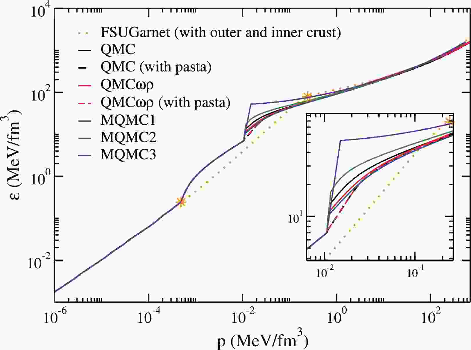
It is expected that the crust thickness and constitution would affect the second Love number and consequently, the tidal polarizability. The neutron star crust is usually divided into two different parts: the outer crust and the inner crust. Piekarewicz and Fattoyev (2008) [66], investigated the impact of the crust by considering simple expressions. For the outer crust, the region where all neutrons are bound to finite nuclei, a crystal lattice calculation that depends on the masses of different nuclei was performed. For the inner crust, where the pasta phase is expected to exist, the authors used a polytropic EoS that interpolates between the homogeneous core and the outer crust. They concluded that for fixed compactness, the second Love number is sensitive to the inner crust, but given that the tidal polarizability scales as the fifth power of the compactness parameter, the overall impact is minor. In the present work, we use the BPS EoS from Baym et al. (1971) [67] for the outer crust and the pasta phase for the inner crust, and investigate their effects on the deformability of the NS. The difference between the total equations of state (outer crust + inner crust + liquid core) presented here and that used in Piekarewicz & Fattoyev (2008) [66] is evident in Fig. 1. One can see that the outer crusts are coincident and the liquid cores of all the EoS are similar. It should be noted that since the QMC model is not used to calculate the outer crust, we employ EoS found in the literature for this region. A more robust prescription of the outer crust is given in Fantina et al. (2020) [68], and we discuss the difference compared to our work when the results are presented in Section V. Hence, most of the differences observed in Fig. 1 reside in the inner crust and around the crust-core transition region. Notice that the pasta phase is present only in the QMC and QMC
$ \omega\rho $ models. An inset showing the details of the inner crust, where the pasta phase lies, and the transition region from the pasta to the homogeneous phase is also included. Specifically, the pasta region is inside the ranges of$ n_B = (0.40-6.2)\times 10^{-2} $ fm$ ^{-3} $ (QMC model), and$ n_B = (0.45-6.6)\times 10^{-2} $ fm$ ^{-3} $ (QMC$ \omega\rho $ model). In the next section, we obtain results for the second Love number and the tidal deformability. These results are subsequently discussed.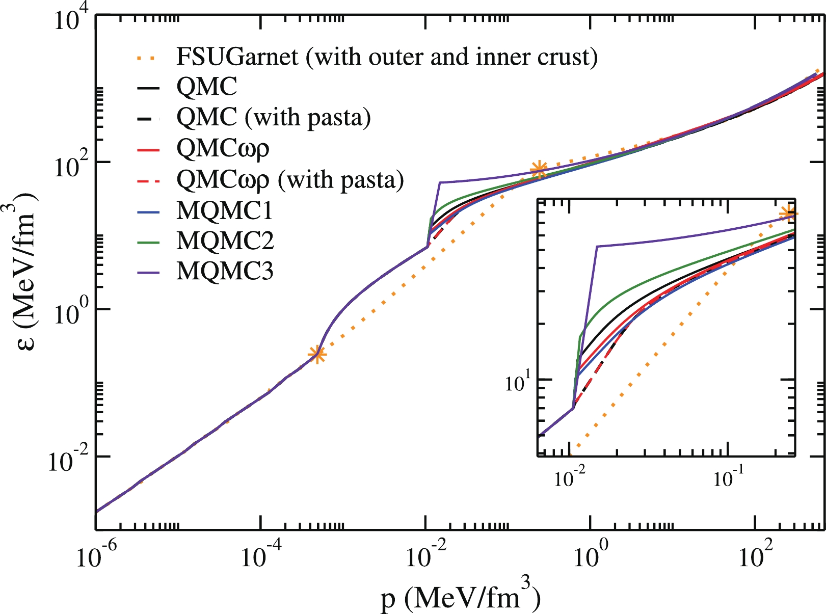
Figure 1. (color online) Stellar matter EoSs described by the QMC and MQMC models in comparison with the FSUGarnet model [66]. The region between the two stars on the orange curve represents the inner crust. Before (after) that region, we have the outer crust (liquid core).
-
We consider the thermal evolution of neutron stars with a composition described by the models discussed in this manuscript. The cooling of neutron stars is governed by the emission of neutrinos from their core, and photons from the surface. All thermal properties of the neutron star from neutrino emission to heat transport depend on their microscopic composition. This is because different compositions lead to different cooling processes, or alter the rate at which certain processes occur. The global properties of stars such as size, mass, and rotation also play an important role in thermal evolution (Franzon et al. (2017) [19]; Negreiros et al. (2012) [29]; (2013) [30]; Yakovlev et al. (2000) [69]; Page et al. (2004) [70]). As such, cooling studies are ideal in terms of bridging the gap between the micro and macroscopic realms of neutron stars.
In recent years, there have been significant advances in the observation of the thermal properties of compact objects (see e.g., Beloin et al. (2018) [71]; Safi-Harb & Kumar (2008) [72]; Zavlin (1999) [73], (2007) [74], (2009) [75]; Pavlov et al. (2001) [76], (2002) [77]; Mereghetti et al. (1996) [78]; Gotthelf et al. (2002) [79]; MvGowan et al. (2003) [80], (2004) [81], (2006) [82]; Klochkov et al. (2015) [83]; Possenti et al. (1996) [84]; Halpern et al. (1997) [85]; Pons et al. (2002) [86]; Burwitz et al. (2003) [87]; Kaplan et al. (2003) [88]; Zavlin et al. (2009); Ho et al. (2015) [89]). The equations that describe thermal energy balance and transport inside a spherically symmetric general relativistic star have been reported by Page et al. (2006) [90], Weber (1999) [91] and Schaab et al. (1996) [92], with (
$ G = c = 1 $ )$ \frac{ \partial (l e^{2\phi})}{\partial m} = -\frac{1}{ \varepsilon \sqrt{1 - 2m/r}} \left( \epsilon_\nu e^{2\phi} + c_v \frac{\partial (T e^\phi) }{\partial t} \right), $

(47) $ \frac{\partial (T e^\phi)}{\partial m} = - \frac{(l e^{\phi})}{16 \pi^2 r^4 \kappa \varepsilon \sqrt{1 - 2m/r}}, $

(48) In Eqs. (47)-(48) l is the luminosity,
$ \phi $ is the metric function, m is the mass as a function of the radial distance r and T is the temperature. In addition to the macroscopic properties obtained from the solution of the Tolman-Opphenheimer-Volkoff (TOV) equations, it is also necessary to calculate the thermal properties that regulate the cooling process. These are the neutrino emissivity ($ \epsilon_\nu $ ), specific heat ($ c_v $ ), and thermal conductivity ($ \kappa $ ). In this work, we consider all established cooling mechanisms for the thermal evolution of neutron stars, and do not consider any exotic processes such as axion cooling (Sedrakian (2016) [93]) and dark matter decay, for instance (Kouvaris (2008) [94]). We now describe the relevant thermal quantities and also refer the reader to Yakovlev et al. (2000) [69] for a thorough review of the subject.The neutrino emissivities are given by the following processes:
● Direct Urca (DU) Process:
$ n \rightarrow p + e^- + \bar{\nu} $ ,$ p + e^- \rightarrow n + e^- + \nu $ .It consists of neutron beta decay and electron capture by the proton. This process is extremely efficient in extracting thermal energy from the neutron star and its emissivity is
$ \epsilon_{DU} \sim 10^{27} T_9^6 $ ergs cm$ ^{-3} $ s$ ^{-1} $ (where$ T_9 = T/10^9 $ K) (Prakash et al. (1992) [95]). This can only occur when the three triangle inequalities$ k_{fi} +k_{fj} \geq k_{fk} $ (where i, j, and k are the baryons and leptons, respectively) are satisfied, to guarantee momentum conservation (Prakash et al. (1992) [95]).● Modified Urca (MU) Process:
$ n + n' \rightarrow p + n' + e^- + \bar{\nu} $ ,$ p+n' + e^- \rightarrow n + n' + \nu $ . The MU is similar to the DU, except it contains a bystander particle (denoted by prime) that facilitates momentum conservation. The phase space reduction also limits the efficiency of such a process (compared to the DU). The emissivity of the MU is$ \epsilon_{MU} \sim 10^{21} T_9^8 $ ergs cm$ ^{-3} $ s$ ^{-1} $ . We note here that we adopted the MU emissivities as calculated in (Friman & Maxwell (1979) [96]). It should be noted, however, that it has been reported that medium effects due to pions at higher densities may alter such emissivities (Migdal et al. (1990) [97]; Schaab et al. (1997) [98]; Blaschke et al. (2004) [99]; (2013) [100]).● Bremssthralung (BR) process:
$ n + n' \rightarrow n + n' +\nu + \bar{\nu} $ ,$ n + p' \rightarrow n + p' +\nu + \bar{\nu} $ ,$ p + p' \rightarrow p + p' +\nu + \bar{\nu} $ .These scattering processes have also been calculated in Friman & Maxwell (1979) [96] and have emissivities of
$ \epsilon_{nn} \sim 10^{19} T_9^8 $ ergs cm$ ^{-3} $ s$ ^{-1} $ ,$ \epsilon_{np} \sim 10^{20} T_9^8 $ ergs cm$ ^{-3} $ s$ ^{-1} $ and$ \epsilon_{pp} \sim 10^{20} T_9^8 $ ergs cm$ ^{-3} $ s$ ^{-1} $ .● Pair Breaking and Formation (PBF) process:
$ \{ BB \} \rightarrow B + B +\nu + \bar{\nu} $ ,$ B + B \rightarrow \{ BB \} +\nu + \bar{\nu} $ .(B stands for the baryon in question)
This process is associated with the breaking and formation of pairs as the temperature approaches the critical temperature for pair formation. This process is transient by definition, and only occurs near the onset of pairing. The emissivity depends on the type of pairing, wherein
$\epsilon_{\rm PBF} \sim 10^{21} T_9^7$ ,$\epsilon_{\rm PBF} \sim 10^{22} T_9^7$ , and$\epsilon_{\rm PBF} \sim 10^{21} T_9^7$ for a proton singlet ($ ^1S_0 $ ), neutron singlet ($ ^1S_0 $ ), and neutron triplet ($ ^3P_2 $ ) pairing, respectively (Yakovlev et al. (2000) [69]).It is important to note that these processes are subjected to suppression when the temperature is low enough for pairing to occur. This is due to the presence of an energy gap (
$ \Delta $ ) in the particle energy spectrum. Generally, the emissivities are suppressed by a factor$ \sim e^{-\Delta(T)/T} $ (Levenfish et al. (1994) [25]).For the specific heat, one calculates the contribution of all constituents by employing traditional microscopic calculations, which lead to the specific heat of the species i as,
$ c_{i,v} = \frac{m*_i n_i}{k_{f,i}^2}\pi^2 T, $

(49) where
$ m*_i $ is the effective mass of the i-species. It is important to note that the specific heat is also subject to suppression due to pairing, much like neutrino emission processes, albeit with a more complicated mathematical form (Levenfish et al. (1994) [25]).The final aspect is the thermal conductivity of neutron star matter, which has been thoroughly discussed in Flowers & Itoh (1976) [101]; (1979) [102]; (1981) [103], which has a fit for the high density regime that is given by
$ \kappa \sim 10^{23} \rho_{14}/T_8 $ ergs cm$ ^{-1} $ s$ ^{-1} $ K$ ^{-1} $ (where$ \rho_{14} = \rho/10^{14} $ g/cm$ ^3 $ ).Once we have all the microscopic and macroscopic components, we then solve Eqs. (47)-(48) numerically. To do this, we need two boundary conditions:
● 1.
$ l (r = 0) = 0 $ - which is necessary given that there is no heat flow at the star core.● 2.
$ T_e = T_e(T_b(R)) $ which is the dependence of the effective surface temperature at the star envelope as a function of the mantle ($ T_b $ ) temperature at$ r = R $ . This relationship has been thoroughly investigated by Gudmundsson et al. (1982) [104], (1983) [105]. It accounts for the properties of the star envelope, as well as the possibility of accreted matter due to fallback during the neutron star formation process. -
In this section, we study the effects of the different versions of the QMC and MQMC models on quantities related to gravitational wave observables and neutron star cooling.
-
The results of the tidal deformability
$ \Lambda $ and the Love number$ k_2 $ obtained from the QMC/QMC$ \omega\rho $ models, with and without pasta phases, and the three versions of the MQMC are shown in Fig. 2, with the range for$ \Lambda_{1.4} $ [106] also displayed. In the top and bottom panels of Fig. 2, we display the Love number$ k_2 $ as a function of the compactness of the neutron star, and the variation of$ \Lambda $ with the mass of the star, respectively. As already indicated by Piekarewicz & Fattoyev (2019) [66], the curves do not collapse into a single curve because of their different dependences on y. When the same models are used to compute the tidal polarizability, their differences are enhanced and only two models, namely, QMC$ \omega\rho $ and MQMC3, give results that are consistent with LIGO results for the canonical star. The pasta phase plays a very modest role and its influence is practically unnoticed, which is evident if one compares the curves obtained from QMC with and without pasta and QMC$ \omega\rho $ with and without pasta. Considering the outer crust, all prescriptions, namely, BPS, crystal lattice calculations presented in Piekarewicz & Fattoyev (2019) [66] and the state-of-the-art calculations in Fantina et al. (2020) [68] (tested, but not shown in this work) result in practically the same tidal deformabilities.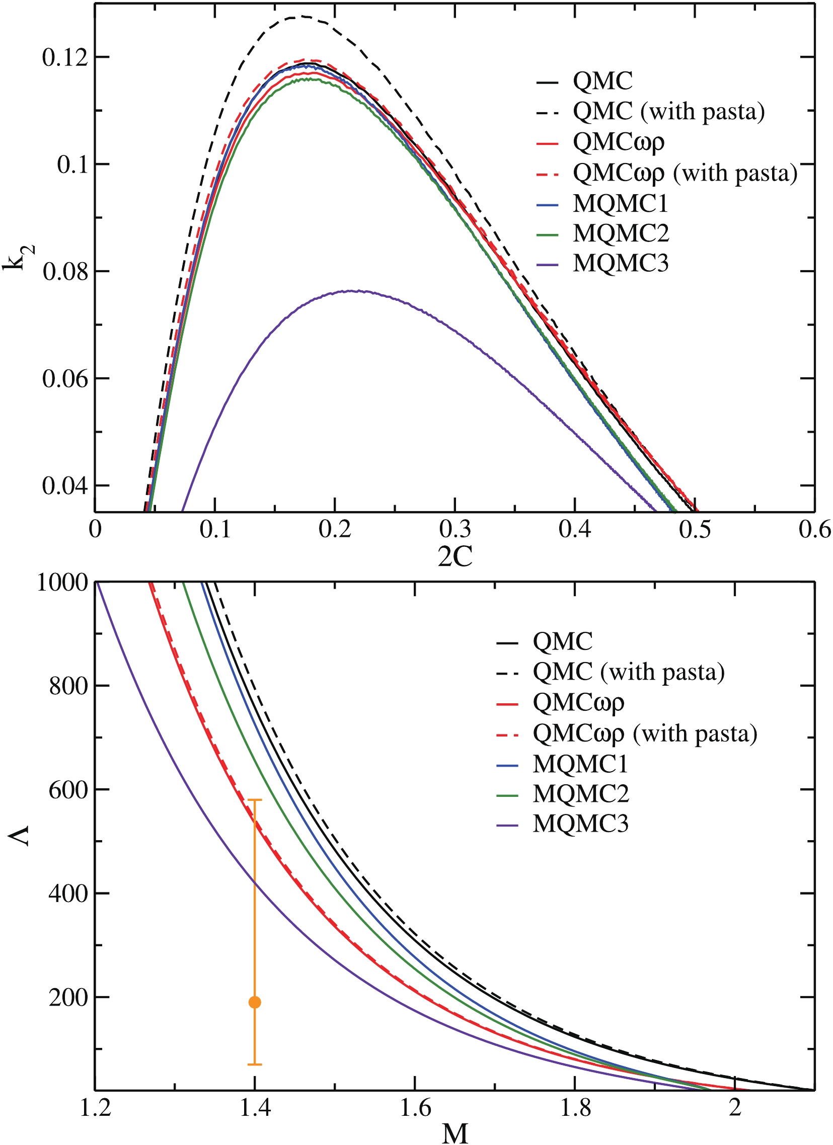
Figure 2. (color online) (top)
$k_2$ as a function of the neutron star compactness, and (bottom)$\Lambda$ as a function of M. Full circle: recent result of$\Lambda_{1.4}=190_{-120}^{+390}$ obtained by LIGO and Virgo Collaboration [106].In recent literature, significant effort has been directed towards constraining the radius of the canonical neutron star, see for instance, Malik et al. (2008) [60], Most et al. (2018) [107], Raithel et al. (2018) [108] and Annala et al. (2018) [109] for studies in which the outcomes of the GW170817 event are used to infer the radius. In Malik et al. (2008) [60], the authors discussed this constraint in the context of the Skyrme and RMF models, and their calculations suggest a range of
$ 11.82\; \rm{km} \leqslant R_{1.4}\leqslant 13.72\; \rm{km} $ . In Most et al. (2018) [107], the constraint on$ R_{1.4} $ was established based on a large number of EoS with pure hadronic matter, without any phase transition. The authors determined that the value of$ R_{1.4} $ was in the range of$ 12.00\; \rm{km} \leqslant R_{1.4} \leqslant 13.45\; \rm{km} $ , with the most likely value being$ R_{1.4} = 12.39\; \rm{km} $ . The upper limit of this range is compatible with the findings of Raithel et al. (2018) [108], namely, the radius of a neutron star cannot be larger than approximately$ 13 $ km. A similar result was obtained in Annala et al. (2018) [109], in which the authors conclude that the maximal radius of a canonical neutron star is$ 13.6 $ km. Concerning the parametrizations that satisfy the constraint for$ \Lambda_{1.4} $ shown in the bottom panel of Fig. 2, namely, QMC$ \omega\rho $ and MQMC3, it was determined that they predict$ R_{1.4} = 12.83 $ km and$ 12.94 $ km, respectively (see Tables 1 and 2). These values are compatible with the aforementioned results.Quantity Model MQMC1 MQMC2 MQMC3 J /MeV 34.50 30.92 25.00 $L_0$ /MeV

93.20 82.46 64.70 a /fm $^{-3}$ 

0.95 0.95 0.95 $V_0$ /MeV

−92.27 −92.27 −92.27 $G_\sigma^{q2}$ 

5.13 5.13 5.13 $G_\omega^2$ 

8.33 8.33 8.33 $G_\rho^2$ 

14.67 12.18 8.08 $M_{\max}$ (M

$_{\odot}$ )

1.97 1.97 1.97 $R_{M_{\max} }$ /km

11.43 11.34 11.18 $R_{1.4}$ /km

13.55 13.32 12.94 Table 2. Nuclear matter and stellar properties obtained from the parametrizations of the MQMC model. The free parameters are also given.
$G_\sigma^{q2}$ ,$G_\omega^2$ and$G_\rho^2$ are given in$10^{-5}$ MeV$^{-2}$ . For all parametrizations,$B/A=-16.4$ MeV,$n_0=0.15$ fm$^{-3}$ ,$m_q = 210.61$ MeV,$K_0 = 295$ MeV, and$M^*_N/M_N = 0.84$ .In Fig. 3 we show the tidal deformabilities of each neutron star in the binary system.
$ \Lambda_1 $ is associated with the neutron star with mass$ m_1 $ , which corresponds to the integration of every EoS in the range$ 1.37 \leqslant m/M_{\odot} \leqslant1.60 $ , obtained from GW170817. The mass$ m_2 $ of the companion star is determined by solving${\cal{M}}_c = 1.188 M_{\odot} = $ $ \dfrac{(m_1 m_2)^{3/5}}{(m_1+m_2)^{1/5}}$ (Abbott et al. (2017) [111]). We notice that only the QMC$ \omega\rho $ model (with and without pasta phases), and the MQMC3 parametrization yield values between the confidence lines. These specific models satisfy the predictions from the LIGO and Virgo collaboration due to the$ R_{1.4} $ dependence of$ \Lambda_{1.4} $ . The results of several different studies indicate that$ \Lambda_{1.4}\propto R_{1.4}^\alpha $ , but with$ \alpha\ne 5 $ , as implied by Eq. (46). In Lourenço et al. (2019) [110], for instance, in which an analysis of 35 relativistic mean-field models was performed, the authors found$ \alpha = 6.58 $ . Therefore, parametrizations that present lower values of$ R_{1.4} $ , in general, lead to a decrease of$ \Lambda_{1.4} $ . In the case of the QMC/MQMC models, such a decrease favors parametrization to satisfy the constraint shown in Fig. 2 (this is the case for the QMC$ \omega\rho $ and MQMC3 models). Regarding Fig. 3, we identify the points (circles and squares) for which one of the companion stars of the binary system has the value$ m_1 = 1.4M_\odot $ . Therefore, for these points, we have$ \Lambda_1 = \Lambda_{1.4} $ . We can also see from this figure that lower values of$ \Lambda_{1.4} $ , due to the smaller values of$ R_{1.4} $ , also lead to consistency of the curves with the LIGO and Virgo band constraint.
Figure 3. (color online) Tidal deformabilities obtained from the QMC, QMC
$\omega\rho$ and MQMC models for both components of the binary system related to the GW170817 event. The confidence lines (50% and 90%) are the recent results of LIGO and Virgo collaboration taken from Abbott et al. (2018) [106]. The shaded region represents the obtained results with the consistent relativistic mean field models in Lourenço et al. (2019) [110]. Circles (QMC model) and squares (MQMC model): points for which$m_1=1.4M_\odot$ and, consequently,$\Lambda_1=\Lambda_{1.4}$ . -
We now present the results of our thermal evolution studies, obtained based on numerical solutions of Eqs. (47) and (48). We begin by showing the cooling of a set of stars, covering a wide range of masses for the QMC model. They are shown in Fig. 4. As shown in Fig. 4, all stars exhibit fast cooling, characterized by a sharp drop in their surface temperature at the age of
$ \sim 100 $ years. Such fast cooling is the manifestation of a prominent presence of the direct Urca process (DU) in the stellar core, which is indeed the case for these stars. The DU process is extremely efficient in exhausting the star's thermal energy, leading to fast cooling (Prakash et al. (1992) [95]). In turn, this indicates that such thermal evolution is mostly incompatible with observed data (unless the DU process is suppressed), as we discuss in the following.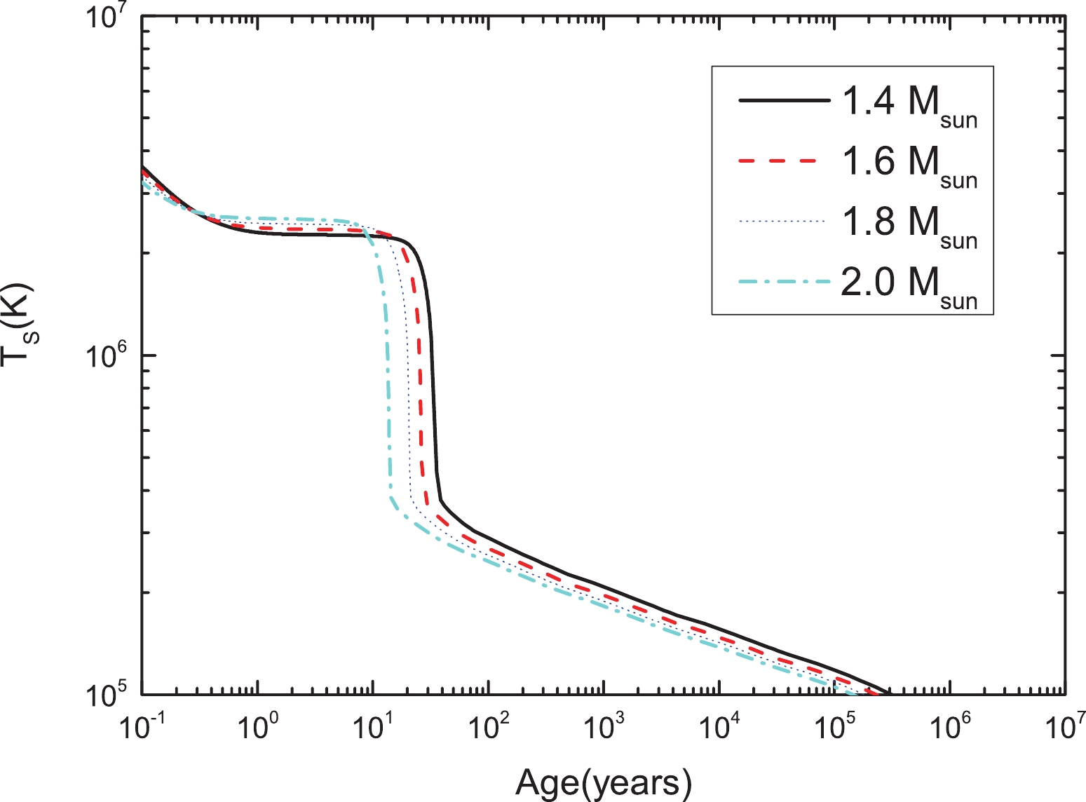
Figure 4. (color online) Thermal evolution of neutron stars described by the QMC model. The y-axis represents the red-shifted surface temperature and x-axis represents the age. Each curve represents the thermal evolution of a neutron star with a different mass. All objects exhibit fast cooling due to prominent DU processes in their core.
In Fig. 5, we show the thermal evolution of QMC neutron stars with the inner crust described by the pasta phase. It is evdent that the pasta phase has little effect on the overall cooling behavior of the star. This is expected because the pasta phase occupies only a small region. Careful analysis leads to the conclusion that the pasta phase had the minor effect of aiding in core-crust thermalization, leading to a core-crust thermal relaxation that is
$ \sim 3.5 $ years faster on average. This seems reasonable, given that the pasta phase smooths the core-crust transition. Thus, it is expected that this will also smooth out heat propagation between these regions. However, we note that these are rough estimates and a more detailed calculation is warranted, in which the thermal and conductivity properties of the pasta phase are explored in more detail.
Figure 5. (color online) Same as in Fig. 4 but for stars with pasta phase in the inner crust.
We now repeat the preceeding calculations, but for the QMC
$ \omega \rho $ model without pasta (Fig. 6) and with pasta (Fig. 7).
Figure 6. (color online) Surface temperature as a function of the age of stars in the QMC
$\omega \rho$ model. Each curve represents the cooling of stars with the indicated mass.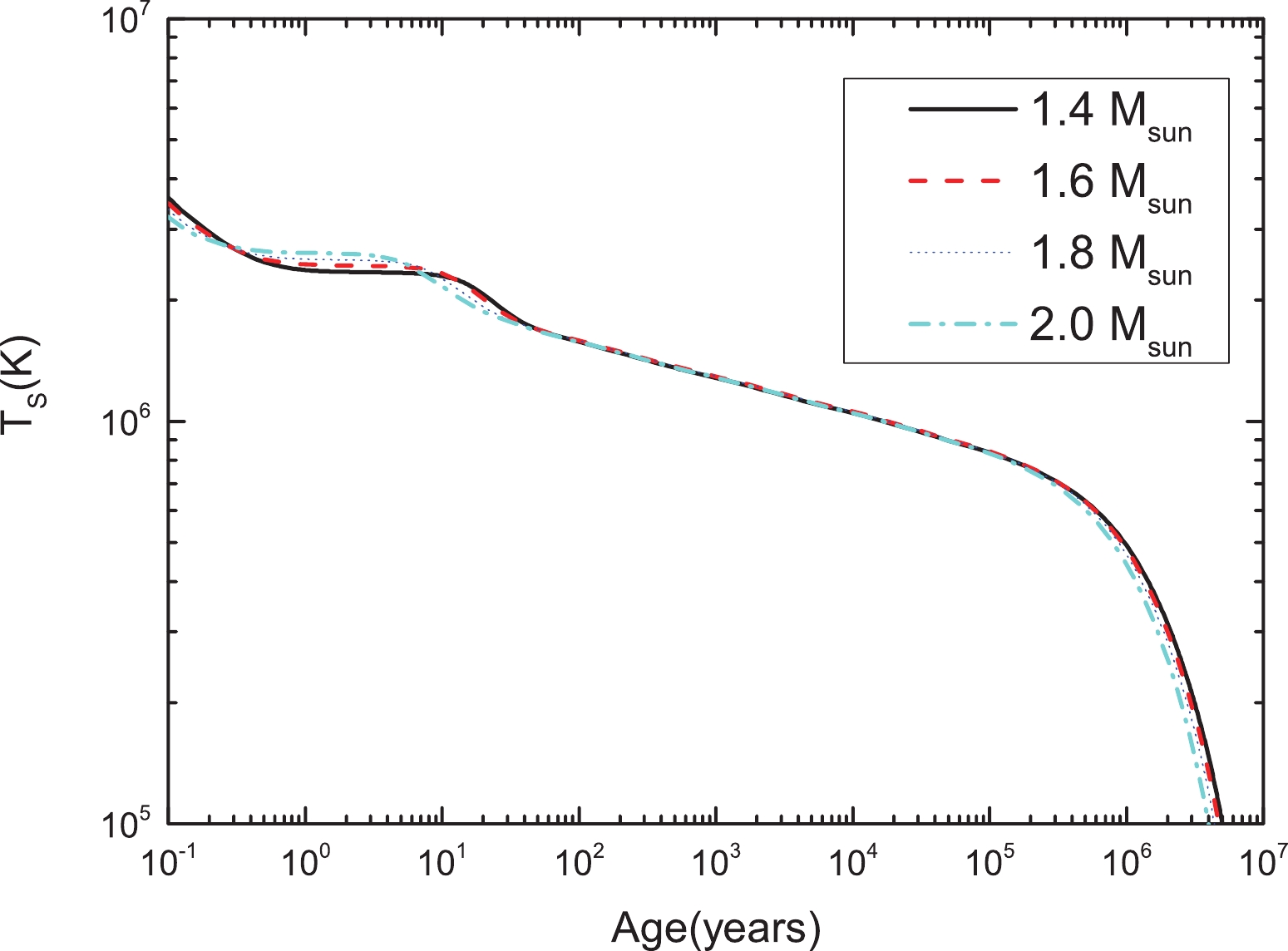
Figure 7. (color online) Same as Fig. 6 but for stars with a pasta phase.
Similar to the previous case (QMC), the pasta phase has little effect on the overall cooling, but instead only delays thermalization by a few years. However, unlike the previous model, all stars exhibit slow cooling in this case, which indicates that there is no sharp drop in temperature when the core and crust are thermally coupled. This is because in this particular model, the proton fraction at the core of the star is low enough to prevent the DU process from occurring, even at the larger densities of heavier stars, thus leading to a substantially slower thermal evolution.
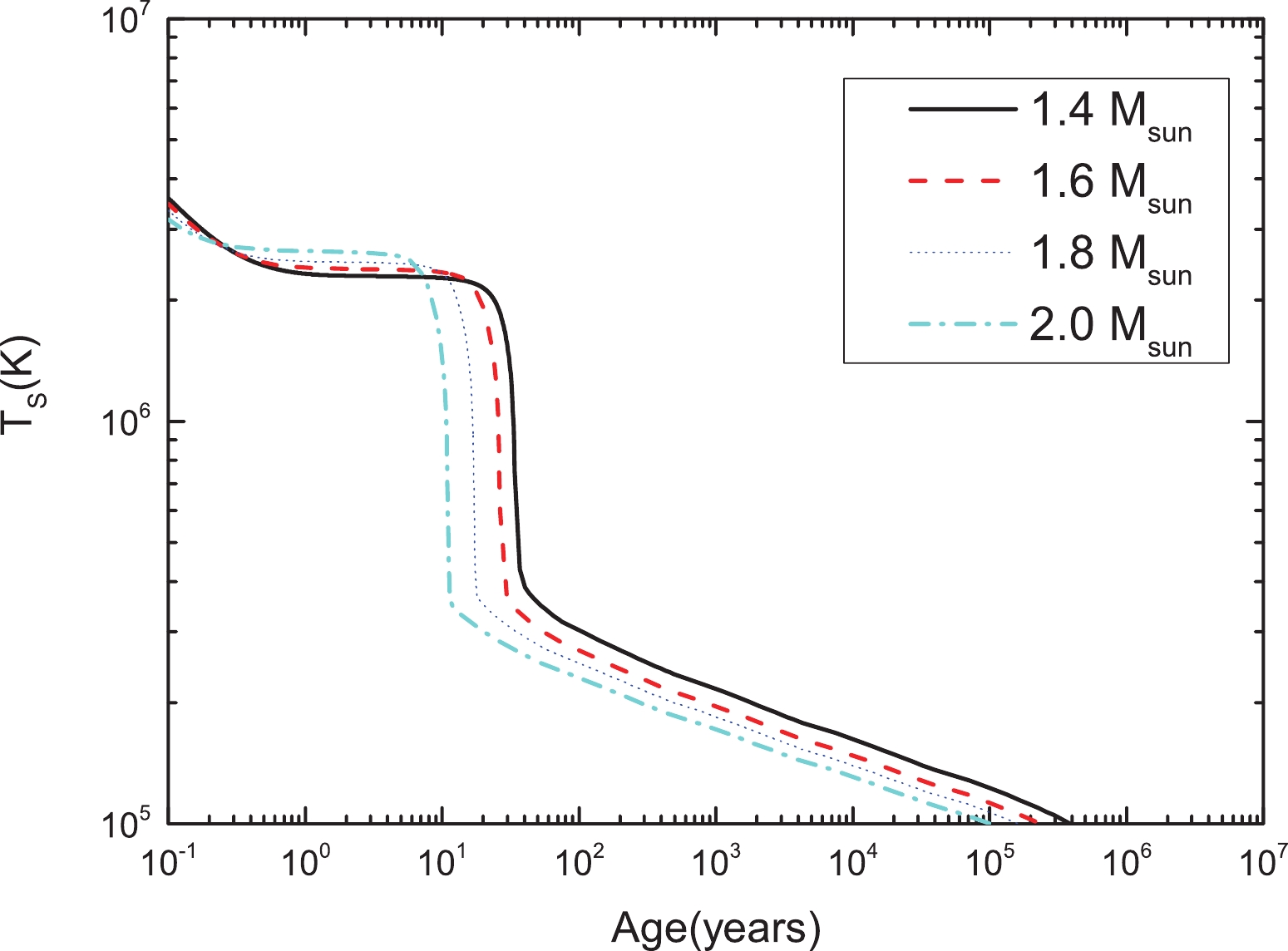
Figure 9. (color online) Same as Fig. 8 but for the MQMC2 model.
We now investigate the cooling of the neutron stars described by the MQMC model to determine if the different prescriptions used in the EoS calculations play a role in this process. In Figs. 8 - 10 , we show the cooling of neutron stars of different masses for the different MQMC models.
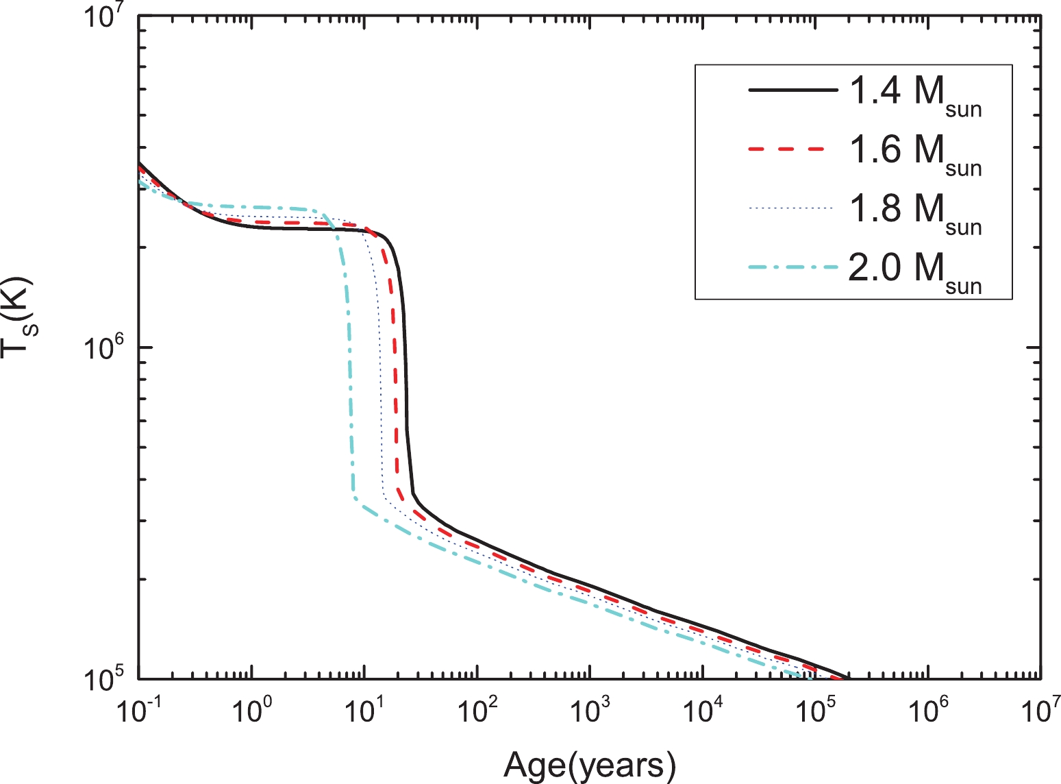
Figure 8. (color online) Thermal evolution of different neutron stars under the MQMC1 model.

Figure 10. (color online) Same as Fig. 8 but for the MQMC3 model.
We can see that from the results shown in Figs. 8 - 10, it is apparent that the overall cooling behavior associated with each model is, qualitatively, the same. For MQMC models 1 and 2, we observe that all stars exhibit fast cooling, with MQMC 3 displaying slow cooling (except for high mass stars). It should be noted that we observe a clear correlation between the slope of the nuclear symmetry energy (
$ L_0 $ ) and a fast/slow cooling behavior, whereby stars with higher$ L_0 $ values exhibit faster cooling (QMC, MQMC1, and MQMC2), and lower$ L_0 $ values lead to a slower cooling scenario (QMC$ \omega \rho $ and MQMC3).So far, in our thermal investigation, we have completely ignored the effects of pairing because we are interested in investigating possible differences in the thermal behavior of the different models, and the inclusion of pairing could potentially obfuscate the results. However, it was observed that all the models behaved similarly, with major differences associated with the different values of the symmetry energy slope rather than specific minutia related to the models. We now need to verify that our model is in agreement with observed data, or at the very least, is comparable to other results in recent literature (Negreiros et al. (2018) [15]; Beloin et al. (2018) [71]; Carvalho et al. (2018) [112]; Dexheimer et al. (2015) [113]; Raduta et al. (2017) [114]). In this regard, we need to include pairing. Pairing in neutron stars may potentially occur in three different ways, neutron-neutron singlets (
$ ^1S_0 $ ), neutron-neutron triplets ($ ^3P_2 $ ), and proton-proton singlets ($ ^1S_0 $ ). Neutron-neutron singlets are formed mainly in the neutron-free region of the crust, whereas their triplet counterparts are mainly formed in the lower density regions of the core. In the case of proton-proton pairs, there is still great uncertainty regarding the depth at which they occur in stars. For a review of pairing in neutron stars, we refer the reader to Yakovlev et al. (2000) [69]. Our implementation of pairing follows the same principles used in Beloin et al. (2018) [71], i.e., given the current uncertainties associated with pairing in high-density neutron star matter, we use thermal observation data of neutron stars to constrain neutron and proton pairing at the neutron star core. This allows us to calculate the pairing effects in neutron star cooling processes [suppression of the DU process, the appearance of Pair-Breaking-Formation (PBF) process near$ T_c $ , and the modification of the specific heat of paired particles (Yakovlev et al. (2000) [69])].For completeness, we have shown the cooling of all the investigated models. For our final cooling (with the inclusion of pairing), and the comparison with observed data, we next focus solely on the models that have satisfied the observational constraints discussed so far, namely, the observed mass and tidal deformability, which are QMC-
$ \omega \rho $ and MQMC3. As shown in Figs. 7 and 10, these models exhibit very different thermal evolution, with QMC$ \omega \rho $ displaying an absence of DU, and thus, very slow cooling. However, MQMC3 exhibits a more balanced behavior, wherein low mass stars display slow cooling while heavier objects cool down faster.Figure 11 shows the thermal evolution of the 1.4 and 2.0
$ M_\odot $ stars for the model MQMC3, with nucleon pairing considered. Intermediate mass stars have thermal evolutions between these curves. Also shown are the most prominent observed data regarding cooling of neutron stars (Beloin et al. (2018) [71]; Safi-Harb & Kumar (2008) [72]; Zavlin (1999) [73], (2007) [74], (2009) [75]; Pavlov et al. (2001) [76], (2002) [77]; Mereghetti et al. (1996) [78]; Gotthelf et al. (2002) [79]; MvGowan et al. (2003) [80], (2004) [81], (2006) [82]; Klochkov et al. (2015) [83]; Possenti et al. (1996) [84]; Halpern et al. (1997) [85]; Pons et al. (2002) [86]; Burwitz et al. (2003) [87]; Kaplan et al. (2003) [88]; Zavlin et al. (2009); Ho et al. (2015) [89]). As expected, nucleon pairing leads to slower cooling rates (associated with the suppression of neutrino emissivities, as previously discussed). Thus, when compared to stars without pairing (see Fig. 10) a warmer object at the same age is obtained. From Fig. 11 we note that to explain most of the observed data, within the confines of the cooling description adopted in this work that makes use of the neutrino emissivities as described by Friman and Maxwell [96], the mass of the stars must be within the interval 1.4-1.8$ M_\odot $ (the latter represented by the cyan curve in Fig. 12). However, it is also apparent that there are a few stars below this curve, in which case their mass would be slightly above 1.8$ M_\odot $ . This indicates a group of observed stars within a small mass window, which may be unlikely. Thus, this poses a challenge in terms of describing the data based on the Friman and Maxwell description for the Urca process.The objects that fall above the expected range can be explained by considering fallback in the early stages of neutron star evolution (Gudmundsson et al. (1983) [105]). Such fall back alters the composition of the atmosphere from pure iron to other elements, which affect the thermal evolution, which keeps the star warmer for longer.
Figure 11. (color online) Thermal evolution of a set of stars with different masses for the MQMC3 model, under the effect of nucleon pairing, as well as the observed thermal data of thecooling neutron stars.

Figure 12. (color online) Thermal evolution of a set of stars with different masses for the MQMC3 model with pairing, and taking into account different atmosphere compositions (represented by the amount of accreted matter
$\Delta M/M$ ). The blue hashed region represents the different possible thermal evolutions that encompass different masses and different atmospheric compositions.Figure 12 shows the thermal evolution of stars for the MQMC3 model with pairing, as well as the different possibilities of fallback accretion (
$ \Delta M/M = 10^{-9} $ and$ 10^{-11} $ ). The hashed band represents the different possible thermal evolutions that encompass different masses and different possible atmospheres.Based on the results of Figs. 11 and 12 , we can now conclude that the MQCM3 model not only complies with the constraints set by neutron star mass measurements, and those extracted from tidal deformability, but it is also in agreement with the thermal data of neutron stars.
We now consider the QMC
$ \omega \rho $ (pasta) model, for which the cooling of 1.4 and 2.0$ M_\odot $ stars under the effect of pairing is shown in Fig. 13. As was the case for stars without pairing (Fig. 6), stars in this model exhibit slow cooling. The occurrence of pairing broadens the cooling "spectrum" (which indicates the different cooling tracks associated with stars of different masses), but it still excludes a large portion of observed data.
Figure 13. (color online) Thermal evolution of the 1.4 and 2.0
$M_\odot$ stars of model QMC$\omega \rho$ (pasta), under the effect of nucleon pairing, as well as observed thermal data of cooling neutron stars.For completeness, we also investigate the effect of different atmospheric compositions of the stars of the QMC
$ \omega \rho $ (pasta) model under the effect of pairing, which is shown in Fig. 14. As was the case for the pure iron atmosphere, the thermal evolution of stars in this model is too slow to satisfactorily explain all the data, and fails to describe the observed temperature of colder stars.
Figure 14. (color online) Thermal evolution of stars under QMC
$\omega \rho$ (pasta) model with pairing, and considering different atmospheric compositions (represented by the amount of accreted matter$\Delta M/M$ ). The blue hashed region represents the different possible thermal evolutions that encompass different masses and different atmospheric compositions. -
In the present work, we used five different versions of the quark-meson coupling model to compute the Love number and tidal polarizability. We evaluated them using GW170817 constraints and also investigated the cooling process associated with them. Two of the models were based on the original bag potential structure (QMC model) and three versions considered a harmonic oscillator potential to confine the quarks (MQMC model). The bag-like models also utilized the pasta phase to describe the inner crust of neutron stars. Although they were based on different concepts, all versions of the quark-meson coupling model used in the present work were chosen because they satisfy nuclear bulk properties within acceptable ranges. We compared our EoS with FSUGarnet (Piekarewicz & Fattoyev (2019) [66]) and confirmed that the outer crusts were coincident, and the liquid cores corresponding to all EoS were very similar. Most of the differences were observed for the inner crust and in the vicinity of the crust-core transition region, where the pasta phase was included. Our results indicated that the pasta phase only played a minor role in the calculation of the dimensionless tidal polarizability and just two of the models (QMC
$ \omega\rho $ and MQMC3) yielded results that lie within the expected range of the canonical star$ \Lambda_{1.4} $ . Moreover, it appeared inside the region delimited by the confidence lines. We emphasize that there is a correlation between the model symmetry energy slope and the fact that it satisfied the investigated constraints (or not), such that the lower values appeared to be more consistent with the observational data. Furthermore, we observed that the two models that satisfied the LIGO and Virgo predictions exhibited similar patterns for the radii and polarisability of the canonical star. It is known (Lourenço et al. (2019) [110]) that in general, parametrizations that present lower values of$ R_{1.4} $ lead to a decrease of$ \Lambda_{1.4} $ . Among the examined models, QMC$ \omega\rho $ and MQMC3, which have lower values of$ \Lambda_{1.4} $ , were consistent with the LIGO and Virgo band constraints. It should be noted that the chirp mass value was updated to$ {\cal{M}}_c = 1.186 M_{\odot} $ (Abbott et al. (2019) [115]) after this work was completed, but new calculations for$ m_2 $ do not affect our main results and conclusions.We used the same models to study the cooling process and verified that in this case, there was a clear correlation between the slope of the symmetry energy and the velocity of the cooling process, i.e., models with higher (lower) slope values produced fast (slow) cooling. We note that this result seems to agree with an analysis performed by Dexheimer et al. (2015) [113], in which the authors updated the non-linear
$ \sigma $ model. In this work, a similar trend was observed, i.e. models with larger slope values for the symmetry energy exhibited faster cooling compared to their counterparts with lower values. Once again, the pasta phase played a minor role in cooling by speeding up the process in approxiately 3.5 years, if superconductivity is not considered.We further explored thermal evolution under a more realistic scenario in which nucleon pairing and different atmospheric models were considered. By considering such phenomena, we calculated the thermal evolution of the two models (MQMC3 and QMC
$ \omega \rho $ ) , which was in agreement with the constraints set by the neutron star mass measurements, as well as the tidal deformability estimates from GW170817. Our results were evaluated using observed thermal data on cooling neutron stars, which showed that the MQMC3 model can successfully explain the entire set of observed data (by encompassing the different possible masses and atmospheric compositions). However, model QMC$ \omega \rho $ could only match the observations of high temperature neutron stars, excluding cold objects from its prediction range. However, it is important to note that there is still a need for further investigations, by considering for instance, medium corrections to the modified Urca process (Migdal et al. (1990) [97]; Schaab et al. (1997) [98]; Blaschke et al. (2004) [99]; (2013) [100]) as well as the effects of pairing on the electron thermal conductivity [116]. We intend to pursue these investigations in future research.The results of our studies revealed that among the five investigated models, the only model that can describe astrophysical quantities as massive NS and tidal polarizabilities, in addition to providing an excellent description of the possible cooling processes, is the MQMC3 model. However, more observational data is desirable. It is also important to note that this conclusion was made by considering neutrino emissivities based on calculations by Friman and Maxwell [96]. A different approach for the Urca emissivity by considering medium corrections, as previously indicated, could potentially lead to different conclusions. It should be noted that the adoption of a purely nucleonic EoS such as the one adopted in this work is typical (see the recent works from Bauswein et al. (2019) [117] and Lucca & Sagunski (2019) [118], for instance). However, this does not imply that the consideration of other phases of matter such as quark matter is unusual. There are many other avenues that involve strongly interacting matter that may still be considered in the context of our work. For instance, stellar matter consisting of hadronic and quark EoS with or without a mixed phase, and at higher densities, deconfined quark matter in the CFL and CCS phases (Lau et al. (2017) [119]). It has recently been shown that the existence of quark cores inside massive stars should be considered as the standard pattern and not an exotic alternative (Annala et al. (2020) [120]). This conclusion was based on a model-independent analysis of the sound velocity in both hadronic and quark matter. Hence, once the possibilities of these different phases are considered, the internal constitution affects the quantities investigated in the present work, and every case is worth investigating and examining using observational constraints. The NICER telescope [121] that was launched in 2017 is expected to test theories in nuclear physics by exploring the exotic states of matter within neutron stars using rotation-resolved X-ray spectroscopy and will provide precise values for masses and radii. If this data is integrated with future GW results, the identification of the inner constituents of neutron stars in a binary system (neutron-neutron, neutron-hybrid or hybrid-hybrid) (Christian et al. (2019) [122]) will be possible. The inclusion of other internal phase transitions and their consequences on the thermal evolution of neutron stars is left to future studies. In that sense, the present work is the first step towards calculations related to the pasta-like phase that may be present between hadronic and quark matter in hybrid stars at high stellar densities.
-
D.P.M. thanks Dr. Prafulla K. Panda for useful comments and discussions on the parametrizations of the QMC model and Thomas Carreau and Francesca Gulminelli for providing their outer crust EOS used for tests and comparisons with the results presented in this work.
Neutron star cooling and GW170817 constraint within quark-meson coupling models
- Received Date: 2020-03-20
- Accepted Date: 2020-09-27
- Available Online: 2021-02-15
Abstract: In the present work, we used five different versions of the quark-meson coupling (QMC) model to compute astrophysical quantities related to the GW170817 event and the neutron star cooling process. Two of the models are based on the original bag potential structure and three versions consider a harmonic oscillator potential to confine quarks. The bag-like models also incorporate the pasta phase used to describe the inner crust of neutron stars. With a simple method studied in the present work, we show that the pasta phase does not play a significant role. Moreover, the QMC model that satisfies the GW170817 constraints with the lowest slope of the symmetry energy exhibits a cooling profile compatible with observational data.


 DownLoad: