


 Abstract
 HTML
HTML Reference
 Related
 PDF
PDF


-
Meson decay constants are important nonperturbative quantities for the study of meson leptonic decays, and their results from lattice quantum chromodynamics (QCD) have received considerable attention. The pseudoscalar meson decay constants (
$ f_P $ ) can be effectively used to determine the Cabibbo-Kobayashi-Maskawa (CKM) matrix elements, if combined with experimental measurements of the corresponding leptonic decays. The newest lattice QCD average of$ f_P $ can be found in the review by the Flavor Lattice Averaging Group (FLAG) [1].In principle, vector meson decay constants,
$ f_V $ , can also be used to determine the CKM matrix elements; however, experimental measurements of the leptonic decays of vector mesons are much more difficult than those of pseudoscalar mesons due to small branching ratios. With increasing statistics, the leptonic decay of$ D_s^* $ may be expected to be measured via BES-III or Belle II for the first time in the near future for a vector meson [2]. Then, the comparison of$ f_{D_s^*} $ from experimental and theoretical calculations can be used to study the low energy properties of QCD.Furthermore, the decay constants of heavy-light vector mesons can be used to test the accuracy of the heavy quark effective theory (HQET). By neglecting the terms of
$ {\cal{O}}(1/m_Q) $ , where$ m_Q $ is the heavy quark mass, one can obtain$ f_V/f_P = 1-2\alpha_s(m_Q)/(3\pi) $ [3] from the leading order QCD calculation, which implies that the$ f_V/f_P $ ratio approaches one since the strong coupling constant$ \alpha_s(m_Q) $ vanishes in the infinite heavy quark mass limit. We can obtain the corrections from the higher order terms in charmed mesons through$ f_V/f_P $ from lattice QCD calculations. Moreover, the$ f_V/f_P $ ratios for charmed mesons are input parameters for QCD factorization studies of charmed nonleptonic B meson decays [4, 5]. Another important quantity,$ f_V^T $ , is the coupling of a vector meson to the tensor current. The nonperturbative determination of ratio$ f_V^T/f_V $ is important in the light cone QCD sum rule (LCSR) calculations of form factors in B to vector meson semileptonic decays (see discussions in [6-8]).In this paper, we present a lattice calculation of
$ D_{s}^{(*)} $ ,$ D^{(*)} $ , and$ \phi $ meson decay constants in a lattice setup with chiral fermions, which are usually expected to be important when light flavors are involved, since chiral symmetry is a fundamental property of QCD. We use overlap fermions for valence quarks and carry out the calculation on 2+1-flavor domain wall fermion gauge configurations generated by RBC-UKQCD Collaborations. The lattice size is big enough ($ \sim5.5 $ fm) to prevent large finite volume effects. The light sea quark mass is almost at the physical point. There have been four lattice QCD calculations of$ f_{D_s^*} $ in the literature so far. Two of them were performed on 2-flavor gauge ensembles [9, 10]. The other two were performed on 2+1-flavor ensembles [2] and 2+1+1-flavor ensembles [11], respectively. An unexpected large quenching effect of the strange quark was observed in$ f_{D_s^*} $ and$ f_{D_s^*}/f_{D_s} $ from the 2-flavor result [9] (confirmed in [12] but with a reduced effect), whereas the 2-flavor result from [10] demonstrated a much less pronounced effect. In this study, we develop an independent 2+1-flavor calculation for$ f_{D_s^*} $ for comparison with the aforementioned calculations.The rest of this paper is organized as follows. In Sec. II, we present our framework of the calculation, including the definitions of the decay constants and the lattice setup. Sec. III presents the details of the analyses and the numerical results and discussions. Finally, we summarize our work in Sec. IV.
-
The decay constant,
$ f_{P} $ , of a pseudoscalar meson P is defined as$ \langle 0 | \bar \psi_1(x) \gamma_\mu \gamma_5 \psi_2(x) |P(p) \rangle = {\rm i} p_\mu f_{P} {\rm e}^{-{\rm i}px}, $

(1) with
$ p_\mu $ being the momentum of the meson. Using the partially conserved axial vector current (PCAC) relation, we can obtain$ f_{P} $ from the matrix element of the pseudoscalar density$ (m_{1}+m_{2})\langle 0 | \bar \psi_1(0) \gamma_5 \psi_2(0) |P(p) \rangle = m_{P}^2 f_{P}, $

(2) where
$ m_{1,2} $ are quark masses, and$ m_P $ is the pseudoscalar meson mass. For overlap fermions, the quark mass and pseudoscalar density$ \bar \psi_1 \gamma_5 \psi_2 $ renormalization constants cancel each other out ($ Z_P = Z_m^{-1} $ ) due to chiral symmetry. This makes$ f_P $ , obtained from Eq. (2), free of renormalization.The vector meson decay constant,
$ f_V $ , is given by the matrix element of the vector current between the vacuum and vector meson V as$ \langle 0|\bar\psi_1(0)\gamma_{\mu}\psi_2(0)|V(p,\lambda)\rangle = m_{V}f_V \epsilon_{\mu}(p,\lambda), $

(3) where
$ \epsilon_{\mu}(p,\lambda) $ is the polarization vector of meson$ V(p,\lambda) $ with helicity$ \lambda $ . We use the local vector current on the lattice to compute the above matrix element for convenience; however, we must also calculate the finite renormalization constant for the local current, which was obtained nonperturbatively in Ref. [13] for our lattice setup.In addition to
$ f_V $ , vector mesons have another decay constant,$ f_V^T $ , which is defined through the following matrix element of the tensor current$ \langle 0|\bar\psi_1(0)\sigma_{\mu\nu}\psi_2(0)|V(p,\lambda)\rangle = i f_V^T (\epsilon_{\mu}(p,\lambda) p_\nu - \epsilon_{\nu}(p,\lambda) p_\mu). $

(4) Here, in the tensor current,
$ \sigma_{\mu\nu} = (i/2)[\gamma_\mu,\gamma_\nu] $ . Since the tensor current has a nonzero anomalous dimension, we will give values of$ f_V^T $ in the commonly used$ {\overline{{\rm{MS}}}} $ scheme and at a scale of$ \mu = 2 $ GeV. The matching factor from the lattice to the continuum$ {\overline{{\rm{MS}}}} $ scheme for the tensor current was presented in Ref. [13]. -
Our calculation is carried out on the gauge configurations of
$ N_f = 2+1 $ domain wall fermions generated by RBC-UKQCD Collaborations [14]. We use the gauge ensemble named 48I, with a lattice size of$ L^3 \times T = 48^3 \times 96 $ and a pion mass of$m^{(\rm sea)}_{\pi} = 139.2(4)$ MeV from the sea quarks. The lattice spacing was determined to be$ a^{-1} = 1.730(4) \;{\rm{GeV}} $ [14]; thus, the spatial extension of the lattice is approximately$ La \sim 5.5 \;{\rm{fm}} $ . The parameters of the configurations are given in Table 1.$ L^3\times T $ 

$~a^{-1}$ (GeV)

$~N_{\rm{conf} }$ 

$48^3\times96~$ 

1.730(4)
45$ am_l^{({\rm{val}})}$ 

0.0017, 0.0024, 0.0030, 0.0060 $ m_\pi/ $ MeV

114(2), 135(2), 149(2), 208(2) $ am_s^{({\rm{val}})} $ 

0.0580, 0.0650 $ am_c^{({\rm{val}})} $ 

0.6800, 0.7000, 0.7200, 0.7400 Table 1. Parameters of the gauge configurations used in this work.
$ am_q^{({\rm{val}})} (q = l,s,c) $ are the valence quark mass parameters in lattice units, and the corresponding pion masses (in MeV) are from Ref. [15]. The physical charm quark mass,$ am_c^{\rm{phy}} $ , is estimated to be approximately 0.73 (see below).We use overlap fermions for valence quarks (as in [13]) to perform a mixed action study. The mismatch of the mixed valence and sea pion masses between the domain-wall fermion and the overlap fermion, measured using
$ \Delta_{\rm{mix}} $ , is$ 0.030(6)(5) $ GeV4 [16], which is very small, reflecting a small partial quenching effect. The multi-mass algorithm of overlap fermions [17] permits calculations of multiple quark propagators at a reasonable cost. We calculate propagators with a range of masses from the light to charm quark on 45 configurations. The valence quark masses,$ am_q^{({\rm{val}})} (q = l,s,c) $ , in lattice units are given in Table 1. The deflation algorithm is adopted to accelerate the inversion by projecting the 1000 low eigenvectors (including zero modes) of the overlap Dirac operator, which are calculated explicitly beforehand.We use four mass parameters,
$ am_l^{({\rm{val}})} $ , (as listed in Table 1) for the light valence quarks for chiral interpolation. The corresponding pion masses range from 114 MeV to 208 MeV [15]. Two strange quark mass parameters are used to extrapolate to the physical strange quark mass point. The bare charm quark masses that we use are approximately$ 0.72 $ in lattice units, which are not small. For chiral lattice fermions, although the discretization error due to the heavy quark mass starts at$ {\cal{O}}((am_c)^2) $ , it could still be large. Thus, we shall try to estimate the finite lattice spacing effects in our results for D-mesons. -
The matrix elements in Eqs. (1), (3), and (4), using which the decay constants are defined, can be derived directly from the related two-point functions, with the currents being the sink operators. Since the mesons involved in this study are all ground state hadrons, for the matrix elements to be determined precisely, it is desirable that the two-point functions be dominated by the contribution from the ground states. In this work, we adopt the Coulomb wall-source technique. In other words, we perform the Coulomb gauge fixing to the gauge configurations first and then, calculate the two-point functions using the following wall-source operators, which are obviously gauge dependent,
$ O^{(W)}_{\Gamma}(t) = \sum\limits_{\vec{y},\vec{z}}^{}\bar \psi ^{f_1}(\vec{y},t) \Gamma \psi ^{f_2}(\vec{z},t), $

(5) where
$ \psi ^{f} = u,d,s,... $ , and$ \Gamma = \gamma_5 $ for pseudoscalar mesons and$ \Gamma = \gamma _i $ ($ i = 1,2,3 $ ) for vector mesons. Based on our experience [15], in addition to the suppression of excited states, the choice of wall source can also suppress the P-wave scattering states in the vector channels.For the sink operators, we use spatially extended operators,
$ O_{\Gamma}(\vec{x},t;\vec{r}) $ , by splitting the quark and anti-quark field with spatial displacement$ \vec{r} $ , namely,$ O_{\Gamma}(\vec{x},t;\vec{r}) \equiv \bar \psi^{f_1}(\vec{x}+\vec r,t) \Gamma \psi^{f_2}(\vec{x},t) $ . The operators with the same spatial separation$ r\equiv\lvert \vec{r} \rvert $ are averaged to guarantee the correct quantum number and also to increase the statistics as a by-product. Thus, the two-point functions that we calculate are$ C_{P}(r,t) = \frac{1}{N_r}\sum\limits_{\vec{x},\lvert {\vec{r}}\rvert = r} \langle 0 | O_{\gamma_5}(\vec{x},t;\vec{r})O^{(W)\dagger}_{\gamma_5}(0)|0\rangle, $

(6) $ C_{V}(r,t) = \frac{1}{3 N_r}\sum\limits_{\vec{x},i,\lvert {\vec{r}}\rvert = r} \langle 0 | O_{\gamma_i}(\vec{x},t;\vec{r})O^{(W)\dagger}_{\gamma_i}(0)|0\rangle, $

(7) and
$ C_T(r = 0,t) = \frac{1}{3}\sum\limits_{\vec x,i}\langle 0 | O_{\sigma_{0i}}(\vec x,t)O^{(W)\dagger}_{\gamma_i}(0)|0\rangle, $

(8) where
$ N_r $ is the number of$ O_\Gamma(\vec x,t;\vec{r}) $ values with the same$ \lvert {\vec{r}}\rvert = r $ . Two-point functions$ C(r,t) $ with different r can be calculated simultaneously without expensive extra inversions. After the insertion of the intermediate states, the spectral expression of a two-point function is$ \begin{aligned}[b] C(r,t) =& \sum\limits_{n,|\vec{r}| = r} \frac{1}{2m_n N_r}\langle 0|O_\Gamma(\vec{0},0;\vec{r})|n\rangle \langle n|O^{(W)\dagger} |0\rangle {\rm e}^{-m_n t}\\\equiv &\sum\limits_n \Phi_n(r){\rm e}^{-m_n t}, \end{aligned}$

(9) where
$ \Phi_n (r) $ is proportional to the Bethe-Salpeter amplitude$ \dfrac{1}{N_r}\displaystyle\sum\limits_{|\vec{r}| = r}\langle 0|O_\Gamma(\vec{0},0;\vec{r})|n\rangle $ for the n-th state. Since the r dependences of$ \Phi_n(r) $ are different for different states in each channel, a proper linear combination of several$ C(r,t) $ values with different r may yield an optimal two-point function$ C(\omega,t)\equiv\displaystyle\sum\limits_{\omega_i} \omega_i C(r_i,t) $ , which is dominated by the ground state.Obviously, the parameterization of Eq. (9) reveals that spectral weight
$ \Phi_n(r = 0) $ is proportional to the matrix element that defines the decay constant of a specific meson state. However, to obtain the decay constant, we need to remove factor$ \langle n | O^{(W)\dagger}_{\Gamma}|0\rangle $ , which is the matrix element of the wall-source operator,$ O^{(W)\dagger} $ , between the vacuum and the meson state and can be derived from the wall-to-wall correlation function$ C^{W}(t) = \langle 0 | O^{(W)}(t)O^{(W)\dagger}(0)|0\rangle. $

(10) -
To extract the meson masses, we apply two fitting strategies. One strategy is applying correlated simultaneous fittings to the correlation functions with different r using one (for vector mesons) or two (for pseudoscalar mesons) mass terms. The function form used in the simultaneous fits is
$ C(r,t) = \sum\limits_{n = 0} \Phi_n(r) \left[ {\rm e}^{-m_n t} + {\rm e}^{-m_n(T-t)} \right], $

(11) where
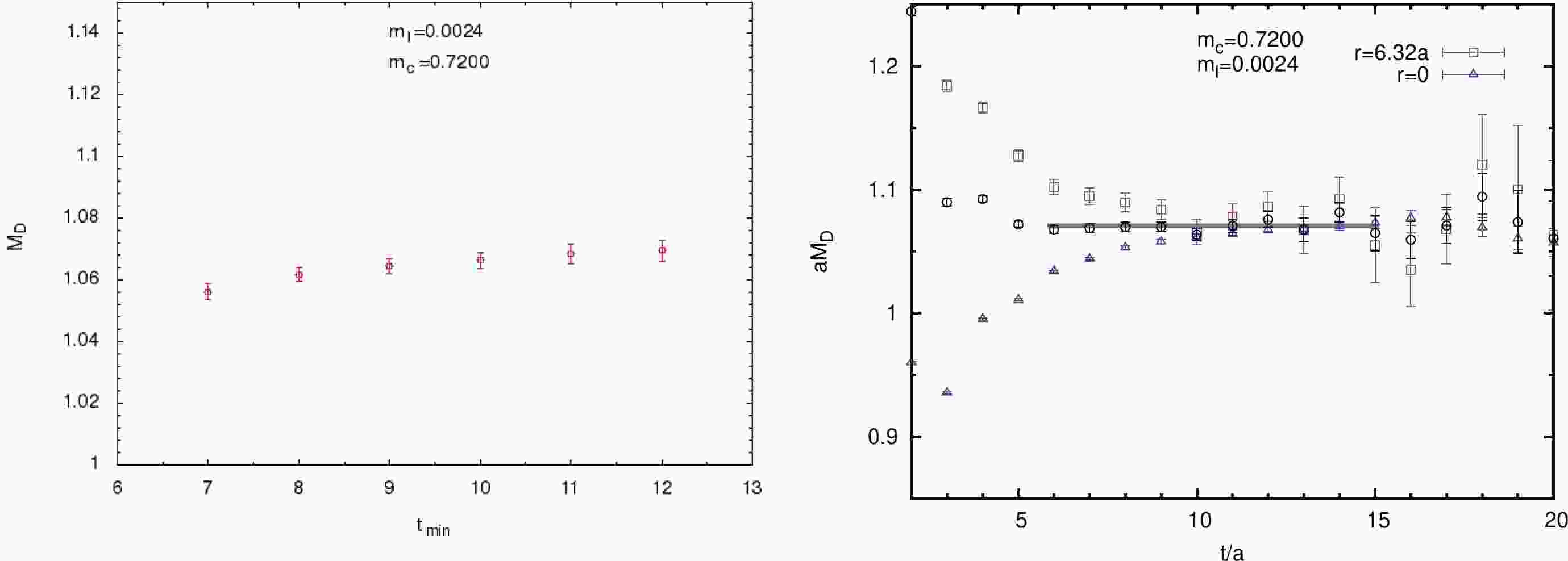
$ T = 96 $ , and the second term in the brackets on the right hand side is obtained from the propagation of the correlator in the negative time direction.$ \Phi_n(r) $ and$ m_n $ are fitted with the minimum$ \chi^2 $ method. We vary the number of mass terms to two or three and check the stability of the fitting results. Within statistical uncertainties, the fitted ground state mass,$ m_0 $ , does not depend on the number of mass terms. The upper limit of fitting range$ [t_{\min}, t_{\max}] $ is chosen using the following criteria. For the pseudoscalar channel,$ t_{\max} $ is fixed to the maximum value where the relative errors of correlators satisfy$ \delta C/C\leqslant $ 5%. For the vector channel,$ t_{\max} $ is chosen by requiring$ \delta C/C\leqslant $ 10%. The lower limit of the fitting range is varied in a wide range during fitting, and we check the stability of the results. Then, among all the fittings that have$ \chi^2/{\rm{dof}}\leqslant 1.0 $ and yield a consistent ground state mass, we choose the earliest$ t_{\min} $ to obtain our final results. The uncertainties are obtained from Jackknife analyses to take into account the correlations among the data as we repeat the fitting for each Jackknife ensemble.In the left panel of Fig. 1, we show fitted ground state mass
$ M_{D} $ in lattice units as a function of$ t_{\min} $ . Here, we finally choose the fitting range [11, 18] for the D meson. In the right panel of Fig. 1, the obtained ground state mass,$ M_{D} $ , (the band in the graph) is compared with the corresponding effective masses,$ M_{\rm{eff}} = \log(C(r,t)/$ $ C(r,t+1)) $ , from various correlators with different r. The data points in the magenta squares are from the correlator with$ r = 6.32a $ ($ \vec r = (2, 6, 0) $ and permutations averaged). The ones in the blue triangles are from the local sink correlator with$ r = 0 $ . The ones in the black circles are the effective masses from a combination of two correlators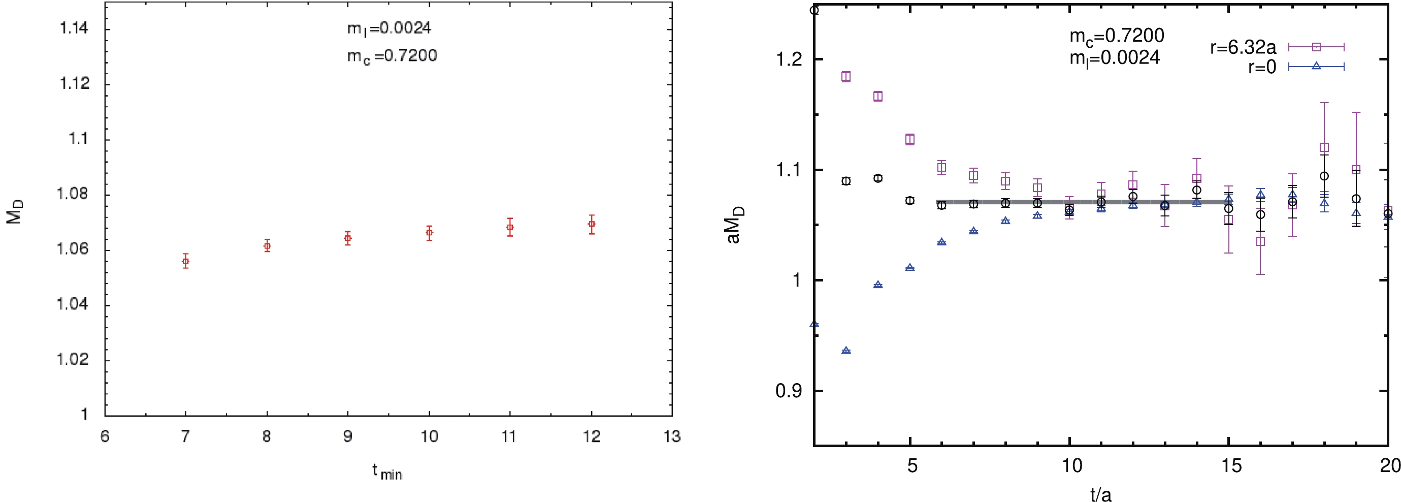
Figure 1. (color online)
$ M_{D} $ in lattice units as a function of$ t_{\min} $ (left panel).$ M_{D} $ (the band in the right graph) from fitting range [11, 18] is compared with the corresponding effective masses from various correlators (right panel).$ C(\omega, t) = C(r = 1, t)+\omega C(r, t), $

(12) where we can tune parameter
$ \omega $ and use various$ C(r, t) $ to make the effective mass plateau from$ C(\omega, t) $ appear as early as possible. This leads to our second fitting strategy. Different states with the same quantum number contribute differently to correlators$ C_\Gamma(r, t) $ , and these contributions vary as r varies. Thus, it is possible to find a large r such that the contribution of the lowest excited state to$ \omega C(r, t) $ cancels that to$ C(r = 1, t) $ , and$ C(\omega ,t) $ is dominated by the ground state.In the right panel of Fig. 1, the black circles present a mass plateau that starts much earlier than that from correlator
$ C(r = 6.32a, t) $ or$ C(r = 0, t) $ . Therefore, we can fit combined correlator$ C(\omega, t) $ easily with a single exponential term. We check that this fitting yields stable and consistent ground state mass as we vary parameter$ \omega $ . We also confirm that the results from the above two fitting strategies are consistent.The fitting results of
$ am_D $ and$ am_{D^*} $ from the two strategies with$ am_c = 0.72 $ are summarized in Table 2 for comparison. The second strategy yields smaller statistical uncertainties, since the mass plateau from the combined correlator appears earlier; thus, data points with less errors are used in fittings. Similar advantages of the second strategy are observed in the analyses of other meson masses; therefore, we adopt strategy II to obtain meson masses in the following.$ am_q $ 

0.0017 0.0024 0.0030 0.0060 $ am_{D} $ 

1.070(4)(1) 1.070(3)(1) 1.070(3)(1) 1.071(3)(1) strategy I 1.071(2)(1) 1.071(2)(1) 1.071(2)(1) 1.073(1)(1) strategy II $ am_{D^*} $ 

1.156(8)(1) 1.157(8)(1) 1.158(7)(2) 1.160(6)(2) strategy I 1.160(2)(1) 1.160(2)(1) 1.160(2)(1) 1.162(2)(1) strategy II Table 2. Masses of D-mesons with
$ am_c = 0.72 $ extracted using the two fitting strategies. The first errors are statistical ones from Jackknife analyses. The second errors are systematic errors from variations in the center values as we vary$ t_{\min} $ . The two strategies yield consistent results.The results of the pion and kaon masses are shown in Table 3. The pion mass and the
$ m_{ss}^2\equiv 2m_K^2- m_\pi^2 $ combination are used to fix the physical up (degenerate with the down quark) and strange quark mass, respectively. From Table 3, we can observe that$ 2m_K^2-m_\pi^2 $ is independent of the pion mass (or equivalently, the up/down quark mass) within the statistical uncertainties. This is exactly what we expect from the lowest-order analysis of the chiral perturbation theory and is the reason we use this combination. The results of the meson masses and decay constants will be interpolated/extrapolated to the physical point where$ (a^2m^2_\pi)^{\rm{phys}} = 0.00651(3) $ and$ a^2m_{ss}^2({\rm{phys}})\equiv a^2(2m_K^2-m_\pi^2)^{\rm{phys}} = 0.1565(6) $ by using$ m_\pi^{\rm{phys}} = 139.6 $ MeV and$ m_K^{\rm{phys}} = 493.7 $ MeV [18]. Here, the uncertainties come from the error of the lattice spacing. Since these uncertainties are much smaller than our statistical error or the discretization error, as we will observe later, we ignore them in our estimate of the systematic uncertainty.$ am_s $ 

$ am_q $ 

$ am_K $ 

$ am_\pi $ 

$ a^2(2m_K^2-m_\pi^2) $ 

0.0580 0.0017 0.2608(24) 0.0659(12) 0.1317(25) 0.0024 0.2621(20) 0.0780(12) 0.1313(21) 0.0030 0.2631(19) 0.0861(12) 0.1310(20) 0.0060 0.2689(20) 0.1202(12) 0.1302(22) 0.0650 0.0017 0.2755(22) 0.0659(12) 0.1475(24) 0.0024 0.2769(22) 0.0780(12) 0.1473(24) 0.0030 0.2780(21) 0.0861(12) 0.1472(23) 0.0060 0.2833(18) 0.1202(12) 0.1461(21) Table 3. Masses of pion and kaon with statistical uncertainties from Jackknife analyses.
In Table 4, we collect the masses of
$ \phi $ and$ K^* $ at our valence quark masses. From the data, we can observe that the mass of$ K^* $ barely depends on the light quark mass with our current statistical uncertainties. To obtain$ m_{K^*} $ at the physical point, we use the following interpolation/extrapolation form:$ am_s $ 

$ am_\phi $ 

$ af_\phi^{\rm{bare}} $ 

$ am_q $ 

$ am_{K^*} $ 

0.0580 0.563(5) 0.126(7) 0.0017 0.505(8) 0.0024 0.504(7) 0.0030 0.503(7) 0.0060 0.504(6) 0.0650 0.579(5) 0.127(7) 0.0017 0.514(7) 0.0024 0.512(7) 0.0030 0.511(7) 0.0060 0.512(7) Table 4. Masses and decay constants of
$ \phi $ and$ K^* $ with the statistical uncertainties. The fitting range of correlators for$ \phi $ is$ t\in [11, 19] $ . The range for$ K^* $ is$ t\in[8, 15] $ .$ m_{K^*}(m_\pi,m_{ss}) = m_{K^*}^{\rm{phys}}+b_1\Delta m_\pi^2+b_2\Delta m_{ss}^2, $

(13) where
$ \Delta m_\pi^2 = m_\pi^2-m_\pi^2({\rm{phys}}) $ , and$ \Delta m_{ss}^2 = m_{ss}^2-m_{ss}^2({\rm{phys}}) $ . This is the Taylor expansion around the physical$ u/d $ and strange quark masses, and we keep only the lowest order, i.e., the linear terms, since our quark masses are close to their physical values. Then, we obtain$ m_{K^*}^{\rm{phys}} = 895(10)\;{\rm{MeV}}, $

(14) where the error includes the statistical/fit uncertainty and the uncertainty of the lattice spacing. Parameter
$ b_1 $ from the fitting is consistent with zero within uncertainty, as expected from the raw data.For the mass of
$ \phi $ , we perform linear extrapolation to physical point$ a^2m_{ss}^2({\rm{phys}}) = 0.1565 $ since we have only two data points, as given in Table 4. For the corresponding$ a^2m_{ss}^2 $ at each of the two strange quark masses, we use the average of the four values in the last column of Table 3. This extrapolation yields$ m_\phi^{\rm{phys}} = 1.018(17)\;{\rm{GeV}} $

(15) with the lattice spacing error included. Both
$ m_{K^*}^{\rm{phys}} $ and$ m_\phi^{\rm{phys}} $ are in good agreement with their experiment values. This means that the finite lattice spacing effects in the study of light hadrons are smaller than our current statistical uncertainties.Vector mesons can decay to two pseudoscalar mesons through P-wave. On our lattice, the minimal nonzero momentum is 226 MeV, which is not small. The thresholds of P-wave decays for
$ \phi $ ,$ D^* $ , and$ D_s^* $ mesons are not open on our lattice, but$ K^* $ can decay to$ K\pi $ on our lattice. We observed mass plateaus for the$ K^* $ meson, but not for the scattering states of$ K\pi $ , which we believe are suppressed by the usage of the Coulomb gauge wall source while calculating the 2-point functions [15]. The agreement of$ m_{K^*}^{\rm{phys}} $ and$ m_\phi^{\rm{phys}} $ (from our interpolation/extrapolation) with their experimental values indicates that it is safe to ignore the threshold effects at our current precision.The masses of
$ D_s $ and$ D_s^* $ mesons are listed in Table 5. We use the experimental value of$ D_s $ (together with$ m_{ss}^2({\rm{phys}}) $ in the above) to set the physical charm (and strange) quark mass. With our lattice spacing, we obtain$ (am_{D_s})^{\rm{phys}} = 1.1378(26) $ by using$ m_{D_s} = 1968.34(7) $ MeV from the Particle Data Group (PDG2018) [18]. We use the following function, similar to Eq. (13), to interpolate/extrapolate$ m_{D_s^*} $ to the physical strange and charm quark mass point:$ am_c $ 

$ am_s $ 

$ am_{D_s} $ 

$ af_{D_s} $ 

$ am_{D_s^*} $ 

$ af_{D_s^*}^{\rm{bare}} $ 

$ f_{D_s^*}^{\rm{bare}}/f_{D_s} $ 

0.68 0.058 1.075(1) 0.139(3) 1.165(3) 0.141(3) 1.011(27) 0.065 1.081(1) 0.141(3) 1.170(3) 0.143(3) 1.008(25) 0.70 0.058 1.095(1) 0.140(3) 1.184(3) 0.141(3) 1.009(27) 0.065 1.102(1) 0.142(3) 1.190(2) 0.143(3) 1.005(26) 0.72 0.058 1.116(1) 0.140(3) 1.204(2) 0.141(3) 1.007(27) 0.065 1.123(1) 0.142(3) 1.209(2) 0.143(3) 1.002(26) 0.74 0.058 1.137(1) 0.141(3) 1.223(2) 0.141(3) 1.004(28) 0.065 1.143(1) 0.143(3) 1.229(2) 0.143(3) 1.000(27) Table 5. Masses and decay constants of
$ D_s $ and$ D_s^* $ with statistical uncertainties. The fitting range of correlators for$ D_s $ is$ t\in [17, 28] $ . The range for$ D_s^* $ is$ t\in[12, 25] $ . The$ f_{D_s^*}^{\rm{bare}}/f_{D_s} $ ratio is collected in the last column.$ m_{D_s^*}(m_{ss},m_{D_s}) = m_{D_s^*}^{\rm{phys}}+b_2\Delta m_{ss}^2+b_3\Delta m_{D_s}, $

(16) where
$ \Delta m_{D_s} = m_{D_s}-(m_{D_s})^{\rm{phys}} $ , and$ b_3 $ is another free parameter. From this, we obtain$ m_{D_s^*}^{\rm{phys}} = 2.116(6)\;{\rm{GeV}}, $

(17) which agrees with the experimental value of
$ 2.1122(4) $ GeV [18]. The interpolation/extrapolation is shown in Fig. 2. The function in Eq. (16) can describe the data very well. The dependence of$ m_{D_s^*} $ on the strange quark mass is relatively small. Therefore, the slope of the straight lines in the left plot of Fig. 2 is small. This is also why the two lines in the right plot are very close to each other. The dependence on the charm quark mass is apparent. The position of the physical point in the left plot indicates that the physical charm quark mass is approximately$ am_c = 0.73 $ .
Figure 2. (color online) Interpolation/extrapolation of
$ m_{D_s^*} $ to the physical point by using Eq.(16).$ am_{D_s^*} $ is plotted as a function of$ a^2\Delta m_{ss}^2 $ (left panel) or$ a\Delta m_{D_s} $ (right panel). The octagon is the result at the physical strange and charm quark mass point.The masses of D and
$ D^* $ mesons are listed in Table 6. The following ansatz is used to interpolate/extrapolate our numerical results to the physical quark mass point:$ am_c $ 

$ am_l $ 

$ am_D $ 

$ af_D $ 

$ am_{D^*} $ 

$ af_{D^*}^{\rm{bare}} $ 

$ f_{D^*}^{\rm{bare}}/f_{D} $ 

0.68 0.0017 1.028(2) 0.122(2) 1.120(3) 0.123(5) 1.01(4) 0.0024 1.029(2) 0.122(2) 1.121(2) 0.123(4) 1.01(4) 0.0030 1.029(2) 0.122(2) 1.121(2) 0.123(4) 1.01(4) 0.0060 1.030(2) 0.123(2) 1.123(2) 0.124(3) 1.01(3) 0.70 0.0017 1.049(2) 0.123(2) 1.140(3) 0.123(5) 1.00(4) 0.0024 1.050(2) 0.123(2) 1.141(2) 0.123(4) 1.00(4) 0.0030 1.050(2) 0.123(2) 1.141(2) 0.123(4) 1.00(4) 0.0060 1.052(1) 0.123(2) 1.142(2) 0.124(3) 1.01(3) 0.72 0.0017 1.071(2) 0.123(2) 1.160(2) 0.123(5) 1.00(4) 0.0024 1.071(2) 0.123(2) 1.160(2) 0.123(4) 1.00(4) 0.0030 1.071(2) 0.123(2) 1.161(2) 0.123(4) 1.00(4) 0.0060 1.073(1) 0.123(2) 1.162(2) 0.123(3) 1.00(3) 0.74 0.0017 1.092(2) 0.123(2) 1.180(2) 0.123(5) 1.00(4) 0.0024 1.092(2) 0.123(2) 1.180(2) 0.123(4) 1.00(4) 0.0030 1.092(2) 0.123(2) 1.180(2) 0.123(4) 1.00(4) 0.0060 1.094(1) 0.124(2) 1.182(2) 0.123(3) 0.99(3) Table 6. Masses and decay constants of D and
$ D^* $ with statistical uncertainties. The fitting range of correlators for D is$ t\in [11, 18] $ . The range for$ D^* $ is$ t\in[10, 16] $ . The$ f_{D^*}^{\rm{bare}}/f_{D} $ ratio is collected in the last column.$ m_{D^{(*)}}(m_\pi,m_{D_s}) = m_{D^{(*)}}^{\rm{phys}}+b_1\Delta m_\pi^2 +b_2\Delta m_{ss}^2+b_3\Delta m_{D_s}. $

(18) Here, the
$ b_2\Delta m_{ss}^2 $ term appears because our lattice results,$ m_{D_s} $ , are not calculated at the physical strange quark mass, and$ m_{D_s}^{\rm{phys}} $ is used to set the physical charm quark mass. We obtain$ m_D^{\rm{phys}} = 1.873(5)\;{\rm{GeV}}\quad {\rm{and}}\quad m_{D^*}^{\rm{phys}} = 2.026(5)\;{\rm{GeV}} $

(19) for the two mesons, respectively, after the interpolations/extrapolations. Our D meson mass agrees with the PDG2018 value of
$ m_{D^\pm} = 1.86965(5) $ GeV within$ 1\sigma $ . However, our$ D^* $ meson mass is heavier than the PDG2018 value of$ m_{D^{*\pm}} = 2.01026(5) $ GeV by approximately 1%. Thus, we estimate the discretization error associated with the large charm quark mass to be approximately 1% in our results for the charmed meson masses. -
Before we delve into the data analyses for the meson decay constants, first, we present the renormalization constants (RCs) for the local vector current and the tensor current. The RCs of the quark bilinear operators for our lattice setup (overlap fermions on domain-wall fermion configurations) were calculated nonperturbatively in Refs. [13, 19]. For the 48I ensemble used in this work, we employed both the RI/MOM and the RI/SMOM schemes to calculate those constants nonperturbatively [13]. The matching factors to the
$ {\overline{{\rm{MS}}}} $ scheme for the local axial vector current,$ Z_A $ , and for the tensor current (at a scale of 2 GeV) are listed in Table 7. Because we use chiral fermions, we obtain$ Z_V = Z_A $ , which was also confirmed numerically in Ref. [13].$ Z_A(=Z_V) $ 

$ Z_T/Z_A(2\;{\rm{GeV}}) $ 

$ Z_T(2\;{\rm{GeV}}) $ 

1.1025(16) 1.055(31) 1.163(34) Table 7. Matching factors to the
$ {\overline{{\rm{MS}}}} $ scheme for the local axial vector current and for the tensor current [13]. -
To obtain decay constants
$ f_P $ and$ f_V $ , we perform simultaneous fits to the wall-to-point ($ C_{P/V}(r = 0, t) $ ) and wall-to-wall ($ C^W(t) $ ) correlators for a given meson, M. These fittings are with two exponentials, and the ground state mass is constrained within$ 10\sigma $ to its fitted result from the above strategy II as we determined the meson masses. After removing the matrix element of source operator$ \langle0|O_\Gamma^{(W)}|M\rangle $ from the spectral weight of$ C_{P/V}(r = 0, t) $ , we obtain$ \langle0|O_\Gamma|M\rangle $ and then, decay constants$ f_{P/V} $ by using Eqs. (2), (3) and the fitted meson mass. This fitting and calculation process is repeated for each Jackknife sample to obtain the statistical uncertainty of$ f_{P/V} $ . For$ f_V $ obtained from the local vector current, we need to multiply it with$ Z_V( = Z_A) $ , as discussed in Section IIIB.1. In the following, we use a superscript “bare” to indicate decay constants obtained directly from the local vector current.The bare decay constants
$ f_V $ in lattice units for the$ \phi $ meson at our two strange quark masses are given in the third column of Table 4. The two center values are almost the same, and our statistical uncertainty is large (~6%). Thus, it is difficult to tell the strange quark mass dependence of$ af_{\phi}^{\rm{bare}} $ . If we perform a constant fit to the two numbers, then we obtain$ (af_{\phi}^{\rm{bare}})^{\rm{phys}} = 0.1265(49) $ or$ f_{\phi}^{\rm{phys}} = 241(9) $ MeV after multiplying it with$ 1/a $ and$ Z_V $ . If we perform a linear extrapolation to physical strange quark mass point$ a^2 m_{ss}^2(\rm phys) = 0.1565 $ , then we obtain a value of$ f_{\phi}^{\rm{phys}} = 243.4(1.3) $ MeV. We choose the value with a larger error from the constant fit as our result at the physical point. Therefore, we obtain$ f_{\phi}^{\rm{phys}} = 241(9)(2)\;{\rm{MeV}} $

(20) as our final result, where the second error comes from the difference between the constant fit and the linear extrapolation and is treated as a systematic error.
We use
$ f_{D_s} $ to estimate our discretization error due to the large charm quark mass since we cannot extrapolate to the continuum limit with only one lattice spacing. The decay constant in lattice units$ af_{D_s} $ for all charm and strange quark masses are given in Table 5. One can use the function form given in Eq. (16) (replacing$ m_{D^*_s} $ with$ f_{D_s} $ ) to extrapolate/interpolate our lattice results in Table 5 to the physical charm and strange quark mass point. We find the following:$ af_{D_s}^{\rm{phys}} = 0.144(3)\quad{\rm{ or}}\quad f_{D_s}^{\rm{phys}} = 249(5)\;{\rm{MeV}}. $

(21) The difference in the center values of
$ f_{D_s}^{\rm{phys}} $ calculated in this work and in our previous work (254(2)(4) MeV) [20] is 5 MeV or 2%. Since our previous result was obtained in the continuum limit, we treat this 2% difference as an estimate of the discretization error and assign it to all our decay constants for the charmed mesons in this work.The vector meson decay constant,
$ af_{D_s^*}^{\rm{bare}} $ , from our lattice data is given in the sixth column of Table 5. Again, we use the function form given in Eq. (16) (replacing$ m_{D^*_s} $ with$ f_{D_s^*} $ ) to extrapolate/interpolate our lattice results to the physical charm and strange quark mass point. The fitting is shown on the left panel of Fig. 3. Compared with the case of$ am_{D_s^*} $ the quark mass dependence of$ af_{D_s^*}^{\rm{bare}} $ is difficult to see relative to the large statistical errors.
Figure 3. (color online) Interpolation/extrapolation of
$ f_{D_s^*} $ to the physical point by using the function form given in Eq. (16) (left panel). The right panel shows the interpolation/extrapolation of$ f_{D^*} $ by using function form given in Eq. (18). The quark mass dependence is difficult to see with the relatively big statistical errors. The octagons show the results at the physical strange and charm quark mass point.From the extrapolation/interpolation, we obtain
$ (af_{D_s^*}^{\rm{bare}})^{\rm{phys}} = 0.144(3) $ . Multiplying this number with$ 1/a = 1.730(4) $ GeV and$ Z_V = 1.1025(16) $ , we find$ f_{D_s^*}^{\rm{phys}} = 274(5) $ MeV. Here, the uncertainty includes the errors from the statistics, extrapolation/interpolation, lattice spacing, and$ Z_V $ . If we assign a 2% discretization error, then we finally obtain$ f_{D_s^*}^{\rm{phys}} = 274(5)(5)\;{\rm{MeV}}. $

(22) At each quark mass combination, we obtain the
$ f_{D_s^*}^{\rm{bare}}/f_{D_s} $ ratio as given in the last column of Table 5. The statistical error is from Jackknife, using the Jackknife estimates of$ f_{D_s^*} $ and$ f_{D_s} $ . Then, the ratio is extrapolated/interpolated to the physical quark mass point by using the function form in Eq. (16) (replacing$ m_{D^*_s} $ with the ratio). As a result, we find that$ (f_{D_s^*}^{\rm{bare}}/f_{D_s})^{\rm{phys}} = 0.999(24) $ . Multiplying it with$ Z_V $ and assigning a 2% discretization error, we obtain$ (f_{D_s^*}/f_{D_s})^{\rm{phys}} = 1.101(27)(22). $

(23) Decay constants
$ f_{D} $ and$ f_{D^*} $ and the$ f_{D^*}/f_{D} $ ratio from our lattice data are shown in Table 6. Similar to the above analyses for$ f_{D_s} $ and$ f_{D_s^*} $ , we obtain$ f_{D}^{\rm{phys}} = 213(2)(4)\;{\rm{MeV}},\quad\quad f_{D^*}^{\rm{phys}} = 234(3)(5)\;{\rm{MeV}}, $

(24) $ (f_{D^*}/f_{D})^{\rm{phys}} = 1.10(2)(2). $

(25) Here, the first error comes from statistics and the interpolation/extrapolation to the physical quark mass point by using Eq. (18) with the replacement of
$ m_{D^{(*)}} $ by the decay constants or their ratio. For$ f_{D^*} $ , the error of$ Z_V $ is also included in the first error. The second error is the 2% systematic uncertainty due to finite lattice spacing. As an example, the interpolation of$ f_{D^*} $ to the physical pion mass is shown in the right panel of Fig. 3. Since our four light quark masses are distributed around and close to the physical point (the same is also true for our charm quark masses), the uncertainty of$ f_{D^*} $ at the physical point is smaller than those of the lattice data.Now, we turn to the
$ f_{D_s}/f_D $ and$ f_{D_s^*}/f_{D^*} $ ratios, which reflect the size of SU(3) flavor symmetry breaking. These ratios can be calculated in two ways. One is using our final results for$ f_{D_{(s)}^{(*)}} $ at the physical quark mass point. By doing this, we obtain$ 1.17(4) $ for both ratios. The other way is first calculating these ratios at our nonphysical quark masses and then interpolating/extrapolating them to the physical point by using the function form in Eq. (18). The second method yields$ f_{D_s}/f_D = 1.163(14) $ and$ f_{D_s^*}/f_{D^*} = $ 1.17(2) without including the 2% discretization error. Including this error leads to$ f_{D_s}/f_D = 1.163(14)(23)\quad{\rm{and}}\quad f_{D_s^*}/f_{D^*} = 1.17(2)(2), $

(26) which we take as our final results for the two ratios. These results indicate that the SU(3) flavor symmetry breaking effects have a size of ~17%. Our value for
$ f_{D_s}/f_D $ agrees with the result from the RBC-UKQCD Collaborations in Ref. [21], which uses unitary lattice setups with eight gauge ensembles, including the 48I used in this work. -
Because of the bad signal-to-noise ratio in
$ C_T(r = 0, t) $ , we do not directly determine decay constant$ f_V^T $ , but calculate the ratio$ f_V^T/f_V $ from the ratio of two-point functions:$ \frac{f_V^T}{f_V} = \lim\limits_{t\rightarrow \infty}\frac{C_T(r = 0,t)}{C_V(r = 0,t)}\equiv \lim\limits_{t\rightarrow \infty}R(t). $

(27) The cancelation of statistical fluctuations from the numerator,
$ C_T(r = 0,t) $ , and the denominator,$ C_V(r = 0,t) $ , leads to a better signal for ratio$ R(t) $ , since both two-point functions are calculated on the same gauge ensemble and, thus, are correlated. At the large time limit, the contributions from the higher states to the two-point functions are suppressed by their heavier masses. Then, from Eq. (3) and Eq. (4), one can derive that the ratio approaches$ f_V^T/f_V $ for the ground state since the other factors in the numerator and the denominator cancel out. Fig. 4 shows ratio$ R(t) $ for$ D^* $ and$ D_s^* $ in the left and right panels, respectively. The uncertainties,$ \delta R(t) $ , of the ratio shown in the figure are from Jackknife analyses. As we can observe, this ratio approaches a plateau at large t. We perform constant fits to$ R(t) $ in the range [$ t_{\min} $ ,$ t_{\max} $ ] to obtain$ f_V^T/f_V $ , where$ t_{\max} $ is fixed to the maximum value of t with$ \delta R/R\leqslant $ 10%.$ t_{\min} $ is varied to check the stability of the fitting results. The variation ranges of$ t_{\min} $ are indicated by the red lines in Fig. 4. We make sure that all the fittings yield consistent results. In this way, we find the bare value of$ f_V^T/f_V $ at each quark mass point. As an example, the numerical results of this ratio for$ D_s^* $ are presented in Table 8.
Figure 4. (color online) Ratio of two-point functions,
$ R(t) $ , for$ D^* $ (left panel) and$ D_s^* $ (right panel).$ am_c $ 

0.6800 0.7000 0.7200 0.7400 $ am_s $ 

$ (f_{D_s^*}^T/f_{D_s^*})^{\rm{bare}} $ 

0.0580 0.862(2) 0.865(2) 0.867(2) 0.869(2) 0.0650 0.863(2) 0.865(2) 0.867(2) 0.869(2) Table 8. Bare values of
$ f_{D_s^*}^T/f_{D_s^*} $ at various valence quark masses.Then, we use Eq. (16) and Eq. (18) to interpolate/extrapolate our raw data to the physical quark mass point for
$ f_{D_s^*}^T/f_{D_s^*} $ and$ f_{D^*}^T/f_{D^*} $ respectively. After multiplying the results with renormalization factor$ Z_T/Z_A(2\;{\rm{GeV}}) = 1.055(31) $ in the$ {\overline{{\rm{MS}}}} $ scheme and assigning a 2% discretization uncertainty, we find$ (f_{D_s^*}^T/f_{D_s^*})^{\rm{phys}} = 0.92(3)(2)\quad {\rm{and}}\quad (f_{D^*}^T/f_{D^*})^{\rm{phys}} = 0.91(3)(2) $

(28) at the scale of 2 GeV. Here the first uncertainty includes the errors from statistics and interpolation/extrapolation and the error of
$ Z_T/Z_A(2\;{\rm{GeV}}) $ and is dominated by the error of the renormalization factor. The second uncertainty is from the finite lattice spacing effect. -
We calculated decay constants
$ f_P $ ,$ f_V $ , and$ f_V^T/f_V $ of the charmed and light mesons, including$ D_{(s)}^{(*)} $ and$ \phi $ , by using 2+1-flavor domain wall fermion gauge configurations at one lattice spacing. The valence overlap fermion has 4, 2, and 4 mass values, respectively, for the light, strange, and charm quarks. We use the experimental values of$ m_\pi $ ,$ m_{ss}^2\equiv 2m_K^2-m_\pi^2 $ , and$ m_{D_s} $ to set the physical light, strange, and charm quark masses. The masses of D,$ D_{(s)}^* $ ,$ \phi $ , and$ K^* $ at the physical point are found via interpolation/extrapolation using the lowest order of Taylor expansion (i.e., a linear interpolation/extrapolation) since our valence quark masses are close to their physical values.Masses
$ m_D $ ,$ m_{D_s^*} $ ,$ m_\phi $ , and$ m_{K^*} $ , obtained from our lattice calculation, are in good agreement with their experimental measurements. The$ D^* $ mass we found is 1% higher than its experiment value. The center value of$ f_{D_s} $ from this calculation is 2% away from our previous lattice QCD calculation extrapolated to the continuum limit [20]. Thus, we estimate the discretization uncertainty in this work to be around 2%.The final results of this work for the decay constants are given in Eqs. (20), (22)-(26), (28). By quadratically adding the statistical/fitting uncertainty and the systematic uncertainty, we obtain the decay constants, shown in Table 9, and some of their ratios, shown in Table 10. For light vector meson
$ \phi $ , the statistical error dominates the uncertainties, whereas for the heavy mesons, the discretization error and the error from$ Z_T/Z_A $ (when needed) are the main sources of uncertainty. We believe our results for$ f_{D_s^*}^T/f_{D_s^*} $ and$ f_{D^*}^T/f_{D^*} $ are the first lattice QCD calculations that can be used as input parameters for the LCSR calculations of form factors in B to vector meson semileptonic decays.$ D_s $ 

$ D_s^* $ 

D $ D^* $ 

$ \phi $ 

$ f_{P/V} $ /MeV

249(7) 274(7) 213(5) 234(6) 241(9) $ f_V^T/f_V $ 

− 0.92(4) − 0.91(4) − Table 9. Decay constants of
$ D_{(s)}^{(*)} $ and$ \phi $ in units of MeV.$ f_V^T/f_V $ is given in the$ {\overline{{\rm{MS}}}} $ scheme at the scale of 2 GeV.$ f_{D^*}/f_D $ 

$ f_{D_s^*}/f_{D_s} $ 

$ f_{D_s}/f_{D} $ 

$ f_{D_s^*}/f_{D^*} $ 

1.10(3) 1.10(4) 1.16(3) 1.17(3) Table 10. Ratios of decay constants for
$ D_{(s)}^{(*)} $ .Our number,
$ f_\phi = 241(9) $ MeV, is lower than the$ N_f = 2 $ lattice simulation result in Ref. [22], which yields$ f_\phi = 308(29) $ MeV. This may be due to the dynamical strange quark effects. Note that our$ f_\phi $ is in good agreement with that in [23], which is also a 2+1-flavor lattice calculation. The experimental value of$ f_\phi $ can be extracted from$ \Gamma(\phi\rightarrow e^+ e^-) = 1.251(21) $ keV [18] by using the relation$ \Gamma(\phi\rightarrow e^+ e^-) = \frac{4\pi\alpha^2_{\rm{em}}}{27m_\phi} f_\phi^2. $

(29) Inputting
$ \alpha_{\rm{em}} = 1/137.036 $ and$ m_\phi = 1019.461(16) $ MeV [18], one finds$ f_\phi^{\rm exp} = 227(2) $ MeV. Our result agrees with the experiment value at$ 1.5\sigma $ .Our value for
$ f_D $ is 213(5) MeV, which agrees with other lattice QCD calculations with 2-flavor [24], 2+1-flavor [25-27], and 2+1+1-flavor [28, 29] simulations. Combining the latest experimental average,$ f_{D^+}|V_{cd}| = 45.91(1.05) $ MeV, from PDG2018 [18] and our$ f_D = 213(5) $ MeV, one obtains$ |V_{cd}| = 0.2155(51)(49). $

(30) Here, the two errors are from the lattice calculation and experiment, respectively.
In Fig. 5, we compare
$ f_{D_{(s)}^*} $ and the$ f_{D_s^*}/f_{D_s} $ ratio from this work and other lattice QCD calculations [2, 9-12]. The values from the 2+1-flavor and 2+1+1-flavor simulations are consistent. There might be tension between the 2-flavor calculations and other calculations, including the dynamical strange quark. This may reflect an unexpected large quenching effect from the strange quark. However, the 2-flavor calculation of$ f_{D_s^*}/f_{D_s} $ in [10] shows that this quenching effect is not as significant as that observed in [9]. The two calculations employ different lattice actions of the two-flavor theory. The computation in [12] is performed on the same 2-flavor gauge ensembles as those used in [9] and employs the same analysis method as that used in [11]. It yields a$ f_{D_s^*}/f_{D_s} $ with a smaller strange quark quenching effect and, therefore, is more in agreement with [10]. Thus, more lattice QCD calculations, especially those with two dynamical flavors, are certainly welcome to clarify this situation.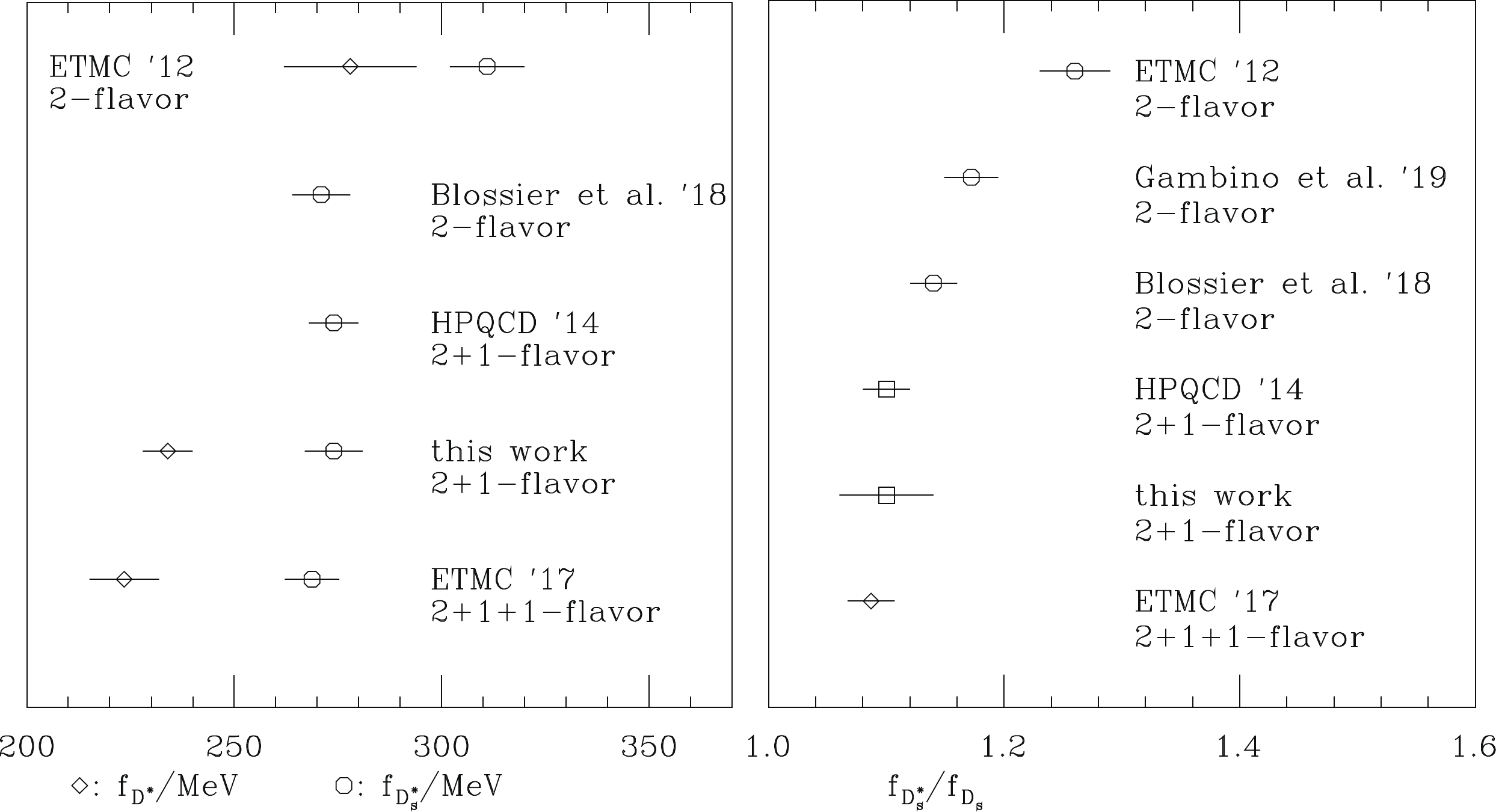
Figure 5. Comparisons of
$ f_{D_{(s)}^*} $ (left panel) and$ f_{D_s^*}/f_{D_s} $ (right panel) from lattice QCD calculations.The ratios of decay constants of charmed mesons in Table 10 show that the size of heavy quark symmetry breaking is approximately 10%, whereas the size of SU(3) flavor symmetry breaking is approximately 17%.
To better control the systematic uncertainty from discretization effects in our work, we need to perform our calculation at more lattice spacings in the future. We also need to include the quark-line disconnected diagram for the
$ \phi $ meson two-point function. To accurately estimate the threshold effects of strong decays of the vector mesons, further studies on larger volumes are necessary. -
We thank RBC-UKQCD collaborations for sharing the domain wall fermion configurations. We also thank the National Energy Research Scientific Computing Center (NERSC) for providing HPC resources that have contributed to the research results reported within this paper.
Charmed and ϕ meson decay constants from 2+1-flavor lattice QCD
- Received Date: 2020-08-22
- Available Online: 2021-02-15
Abstract: On a lattice with 2+1-flavor dynamical domain-wall fermions at the physical pion mass, we calculate the decay constants of


 DownLoad: