


 Abstract
 HTML
HTML Reference
 Related
 PDF
PDF


-
In recent literature [1-3], it has been suggested that there exists a sub-threshold
$ 1/2^- $ nucleon resonance hidden in the$ S_{11} $ channel of$ \pi N $ scatterings, with a pole mass$ \sqrt{s} = (0.895 \pm 0.081) -(0.164 \pm 0.023){\rm i} $ GeV. The result was obtained by using the production representation (PKU representation) for partial wave amplitudes [4-8]. It was later found that the$ N^*(890) $ pole may also be generated from a conventional and simple$ K $ -matrix fit, though the latter suffers from the existence of spurious poles on the first Riemann sheet of the complex$ s $ plane [9]. The properties of$ N^*(890) $ were also investigated, such as its coupling to$ N\gamma $ and$ N\pi $ [10, 11]. It was found that its coupling to$ N\pi $ is considerably larger than that of$ N^*(1535) $ , while its coupling to$ N\gamma $ is comparable to that of$ N^*(1535) $ . The coupling results are reasonable and within expectations, providing further evidence for the existence of$ N^*(890) $ .However, firmly establishing the existence of such a subthreshold resonance remains a difficult task. Besides dispersion relations, the most frequently used tools are perturbation chiral amplitudes and their unitarizations (for a recent review, see Ref. [12]) or (unitarized) resonance models. However, these unitarization techniques are imperfect when used in the study of low energy strong interaction physics, with particular difficulties encountered in their application to partial wave amplitudes with unequal mass scatterings, as will be discussed in detail in this paper. The major difficulties arise at the
$ s = 0 $ point in the$ s $ plane, where chiral expansions break down, as chiral expansions and partial wave projections do not commute when$ s\to 0 $ . The expected decoupling property of heavy resonances, when their masses are set to infinity, is also violated in partial wave amplitudes at$ s = 0 $ , for a purely kinematical reason, in partial wave projections with unequal mass scatterings. The main aim of this paper is to show how the subthreshold resonance persists, irrespective of the various difficulties and uncertainties that remain in the input quantity – the left part of the scattering amplitude.This paper provides further evidence for the existence of
$ N^*(890) $ , by directly finding a pole in the$ S $ matrix element, calculated from the$ N/D $ method. Early studies on low energy$ \pi N $ scatterings using the$ N/D $ method can be found in Ref. [13]. Nevertheless, to the best of our knowledge, no study on the possible existence of a subthreshold resonance exists in the$ N/D $ literature. In our$ N/D $ calculations, no spurious poles were found on the first Riemann sheet. Also, an$ N/D $ calculation faithfully reproduces all input dynamics, as well as kinematical branch point singularities. We therefore believe the$ N/D $ method to be reliable. However, the calculations in existing$ N/D $ studies do generate spurious branch cuts and spurious poles on the second sheet, due to the truncation of numerical integrations. Nevertheless, their effects can be evaluated to verify that the sum of hazardous contributions is negligible in many cases.This remainder of this paper is organized as follows: In Sec. II, a brief introduction to the
$ N/D $ method is given, with a solvable toy model calculation. Also in Sec. II, we provide a review on the production representation, which is helpful for understanding the complexity of the$ N/D $ calculations. A subtlety occurs when using the production representation in dealing with$ \pi $ N scatterings: the dispersion representation for the background contribution to the phase shift must be modified and an additional contribution emerges, which is approximately canceled by the contributions from the two virtual poles located near the end points of the cut, caused by$ u $ channel nucleon pole exchanges. A detailed discussion of this subtlety is included in Appendix A. Sec. III focuses on the singularity structure of partial wave amplitudes at$ s = 0 $ , including the discussion on chiral expansion break down and how high energy contributions enter through an analysis on regge asymptotic behavior of$ T(s) $ when$ s\to 0 $ . Sec. IV is devoted to numerical analyses on how a subthreshold resonance may emerge under various phenomenological inputs. -
The partial wave
$ T $ matrix element is expressed as$ T = {N}/{D}\ , $

(1) where
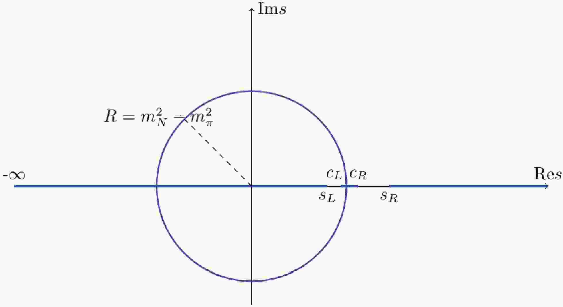
$ D $ contains only the$ s $ -channel unitarity cut or the right hand cut$ R $ , whereas$ N $ only contains the left hand cut ($ l.h.c. $ ) or$ L $ . In Fig. 1,$ R = [s_R, +\infty) $ , whereas$ L $ represents all branch cuts except$ R $ . In Sec. III.B, we will briefly review the determination of the cut structure, as shown in Fig. 1 [14].
Figure 1. (color online) Branch cuts (thick blue lines) of partial wave
$ \pi $ N elastic scattering amplitudes, where$ c_L = {(m_N^2-m_\pi^2)^2}/{m_N^2} $ ,$ c_R = m_N^2+2m_\pi^2 $ .The partial wave unitarity in the single channel is approximated as
$ \mathrm{Im}_R T(s) = \rho(s)\big|T(s)\big|^2\ , $

(2) where
$ \rho = \sqrt{(s-s_L)(s-s_R)}/s, $

(3) with
$ s_L = (m_N-m_\pi)^2 $ ,$ s_R = (m_N+m_\pi)^2 $ , which leads to the following relations:$\begin{aligned}[b] \mathrm{Im}_R[D(s)] = -\rho(s)N(s)\ ,\;\; \mathrm{Im}_L[N(s)] = D(s) \mathrm{Im}_L[T(s)]\ , \end{aligned} $

(4) and subsequent
$ N/D $ equations$ \begin{aligned}[b] D(s) = &1 - \dfrac{s-s_0}{\pi} \int_{R}\dfrac{\rho(s^\prime)N(s^\prime)} {(s^\prime-s)(s'-s_0)}{\rm d}s^\prime \ , \\ N(s) =& N(s_0) +\dfrac{s-s_0}{\pi}\int_L\dfrac{ D(s^\prime) \mathrm{Im}_L[T(s^\prime)]} {(s^\prime-s)(s^\prime-s_0)}{\rm d}s^\prime\ .\end{aligned} $

(5) Notice that when a circular cut appears in
$ T $ on the$ s $ plane, as shown in Fig. 1, the second part of Eq. (4) should be written as$ \mathrm{disc}[N(s)] = D(s) \mathrm{disc}[T(s)] $ . Also, in the second part of Eq. (5), when integration is performed on the circular cut belonging to a subset of$ L $ ,$ \mathrm{Im}_L[T(s)] $ should be replaced by$ \dfrac{1}{2i}\mathrm{disc}[T(s)] $ . After obtaining a numerical solution for Eq. (5), analytical continuation to the complex plane is straightforward: taking$ s $ to be complex while evaluating the integration in Eq. (5), when$ s $ is in the first sheet, and taking$ D^{\mathrm{II}}(s) = D(s)+2{\rm i}\rho N(s)\ ,\quad N^{\mathrm{II}}(s) = N(s)\ , $

(6) when
$ s $ lies on the second sheet. In Eq. (5), the left cut of the partial wave$ T $ matrix element,$ \mathrm{Im}_LT $ , is an input quantity. Throughout this paper, we only discuss$ \mathrm{Im}_LT $ extracted from tree level amplitudes. Hence, with the exception of the case with$ t $ -channel$ \rho $ exchange (as discussed in Sec. IV.B), with an arc cut in the$ s $ plane,$ L $ is always on the real axis. For example, for pure tree level chiral amplitudes,$ L = (-\infty, 0] \cup [c_L,c_R] $ . We will provide a detailed discussion on how to determine$ l.h.c. $ s in Sec. III.B.To solve the integral equations,
$ D $ may be substituted into the second part of Eq. (5) to get$ N(s) = N(s_0) +\tilde B(s,s_0) +\dfrac{s-s_0}{\pi}\int_R \dfrac{\tilde B(s^\prime,s)\rho(s^\prime)N(s^\prime)}{(s^\prime-s_0)(s^\prime-s)}{\rm d}s^\prime\ , $

(7) with
$ \tilde B(s^\prime,s) = \dfrac{s^\prime-s}{2\pi i}\int_L\dfrac{\mathrm{disc}T(\tilde s)}{(\tilde{s} -s)(\tilde{s}-s^\prime)}{\rm d}\tilde{s}\ , $

(8) and use the inverse matrix method to obtain a numerical solution. Throughout this paper, we set
$ s_0 = 1 $ GeV$ ^2 $ , a value slightly below the elastic threshold$ s_R $ .As will become evident later in this paper, there exists a subtlety when using Eq. (5) to discuss unequal mass scatterings. The problem comes from a singularity at
$ s = 0 $ in the partial wave amplitude and in its left cut, which stems from the high energy region$ t\to +\infty $ through the partial wave projections, and also from relativistic spin kinematics. However, before dealing with this problem, we are more interested in finding a solution for Eq. (5) in a simplified toy model, outlined in the following subsection. -
In the
$ N/D $ method, the input quantity is$ \mathrm{Im}_L\, T $ . Let us begin with a simple version of an$ N/D $ study, by assuming$ \mathrm{Im}_L\, T $ is simulated by a set of Dirac$ \delta $ functions, or equivalently,$ \, N = \sum\limits_i\frac{ \gamma_i}{s-s_i}\ , $

(9) which is to be used in the first part of Eq. (5). Therefore, there is no need for a subtraction in the second part of Eq. (5). The
$ T $ matrix, in such a situation, is analytically solvable. We (arbitrarily) set$ Case $ I as one pole at$ s_1 = 0 $ and$ Case $ II as one pole at$ s_1 = -m_N^2 $ and fit to the data obtained from the solutions of the Roy Steiner equations [15] by tuning the parameter$ \gamma_1 $ ; then, we search for poles on the$ s $ -plane. Both cases provide a good fit to the data, and a sub-threshold pole emerges in each case, with a location listed in Table 1. The phase shift and its PKU decomposition [4, 5] are plotted in Fig. 2. In the left panel of Fig. 2, we see the familiar picture that the background cut contribution to the phase shift is concave and negative, while the subthreshold resonance pole provides a positive and convex phase shift above the threshold to counterbalance the former contribution. The sum of the two reproduces the steadily rising phase shift data. In order to better understand this phenomenon, a brief introduction to the production representation of the partial wave elastic scattering$ S $ matrix element is needed.Case I Case II s1 0 $-m_N^2$ 

$\gamma_1/{\rm{GeV} }^2}$ 

0.79 1.34 $\sqrt{s_{\rm pole} }/{\rm{GeV} }$ 

0.810 - 0.125i 0.788 - 0.185i Table 1. Subthreshold pole locations using input Eq. (9).
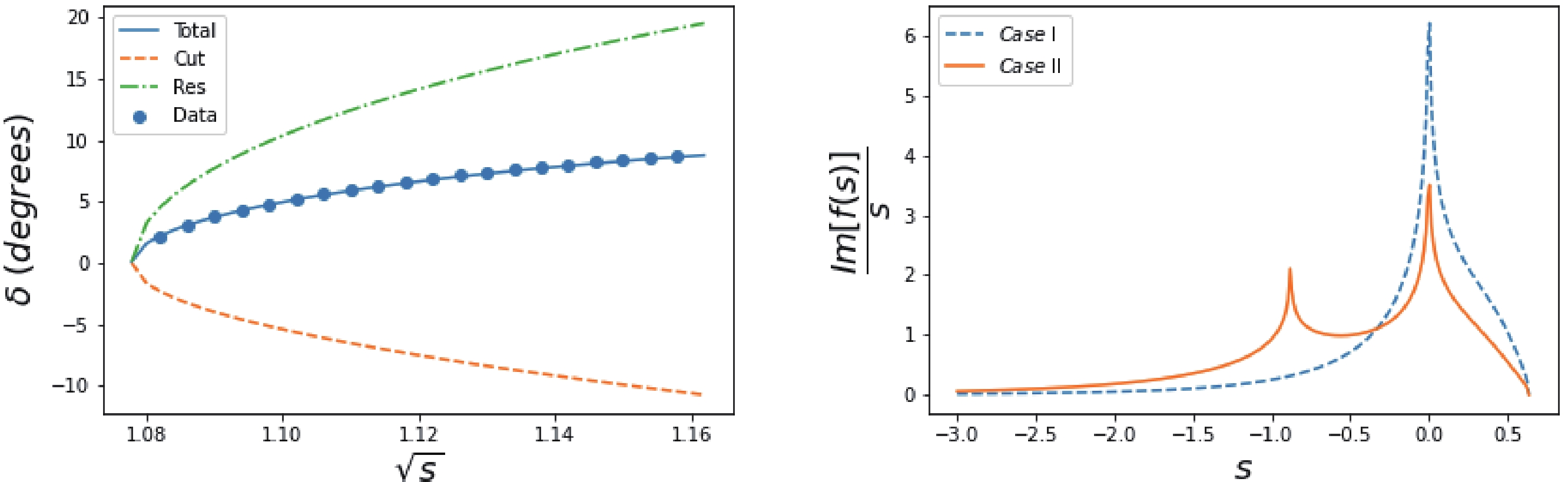
Figure 2. (color online) (left) Fit to the
$ S_{11} $ channel$ \pi $ N scattering phase shift data, taking$ Case $ II as an example (data from Ref. [15]); (right) the spectral function$ \mathrm{Im}_L f(s)/s $ of$ Case $ I and II. Notice that the singularity at$ s = 0 $ in$ Case $ II is due to the kinematical singularity in$ \rho(s) $ defined in Eq. (3), rather than being dynamical. For the definition of different contributions to the phase shift, refer to Sec. II.C. -
The "spectral" function in the r.h.s of Fig. 2 is defined as
$\begin{aligned}[b] f(s) =& \dfrac{s}{{2{\rm i}}\pi}\int_L {\rm d}s^\prime\dfrac{\mathrm{disc}_Lf(s^\prime)/s^\prime }{(s^\prime-s)}\\&+\dfrac{s}{{2{\rm i}}\pi}\int_R {\rm d}s^\prime\dfrac{\mathrm{disc}_Rf(s^\prime)/s^\prime }{(s^\prime-s)}\ , \end{aligned} $

(10) $ \mathrm{disc}_{L,R}f(s) = \mathrm{disc}_{L,R}\left(\dfrac{\ln S(s)}{2{\rm i}\rho(s)}\right)\ , $

(11) where the partial wave
$ S $ matrix element$ S = 1+2{\rm i}\rho T $ , and$ \rho $ is the kinematic factor. In Eq. (10), the integration domain is depicted in Fig. 1, where$ R = [(m_N+m_\pi)^2,+\infty) $ , but the integrand actually disappears in the elastic region, meaning that$ R $ starts from first inelastic threshold. Elastic partial wave$ S $ matrix elements satisfy a production representation of$ S = \prod\limits_iS_i\times {\rm e}^{2{\rm i}\rho(s)f(s)}\ . $

(12) Detailed discussions on how to obtain Eq. (12) can be found in Refs. [4, 5]. The production representation exhibits some beneficial features for our analyses. One advantage is that the phase shifts from different sources are additive, i.e.,
$ \delta(s) = \sum\limits_i\delta_i+\delta_{\rm cut}\ , $

(13) where
$ \delta_i $ comes from the$ i $ -th pole contribution, described by$ S_i $ in Eq. (12). For a resonance located at$ z_0 $ ($ z_0^* $ ) its contribution is$ \delta_{\rm res}=\arctan\left[\frac{\rho(s)sG[z_0]}{M^2(z_0)-s}\right] (S_R={\rm e}^{2{\rm i}\delta_R})\ , $

(14) with
$ G(z_0) = \mathrm{Im}[z_0]/\mathrm{Re}[z_0\rho(z_0)] $ and$ M^2(z_0) = \mathrm{Re}[z_0]+ $ $ \mathrm{Im}[z_0]\mathrm{Im}[z_0\rho(z_0)]/\mathrm{Re}[z_0\rho(z_0)] $ . For a virtual state located at$ s_0 $ ($ s_L<s_0<s_R $ ), its contribution is$ \delta_v=\arctan\left[{\frac{\rho(s)s}{s-s_L}\sqrt{\frac{s_0-s_L}{s_Rs_0}}}\right]\,\,\,(S_v={\rm e}^{2{\rm i}\delta_v})\ . $

(15) For a bound state, the above expression changes sign, i.e.,
$ \delta_b = -\delta_v $ ($ S_b = {\rm e}^{2{\rm i}\delta_b} $ ). The last contribution in Eq. (13), i.e., the background contribution to the phase shift, is$ \delta_{\rm cut}=\rho(s)f(s)\ , $

(16) with the function
$ f(s) $ defined in Eq. (10).The above description of the production representation is in agreement with what has been established in the literature. In our study of
$ \pi $ N scatterings, however, an unexpected new phenomenon occurs. Essentially, the cut structure of the background phase shift,$ \delta_{b.g.} $ , must be modified, due to the presence of the$ u $ -channel nucleon exchange①. As a result, an additional contribution exists in the expression of$ \delta_{b.g.} $ , which is approximately canceled by the contributions from the two newly found virtual poles, located near the end points (i.e.,$ c_L $ and$ c_R $ defined in Fig. 1) of the segment cut, induced by the$ u $ channel nucleon exchange. A more detailed explanation is provided in Appendix A.The additive property of the phase shift contributions is vital in tracing the physical origin of the phase shift. As has been stressed repeatedly, the positive value of
$ \mathrm{Im}_L f(s)/s $ guarantees that the background contribution to the phase shift will be negative and concave, and hence, an isolated singularity on the second sheet is needed to manage the steady rise of the near threshold phase shift. The circular cut caused by$ t $ -channel exchanges and the$ u $ -channel cut (combined with effects of two virtual poles) are not considered here; nevertheless, they are numerically smaller than the cut lying on$ (-\infty, s_L] $ (previous examples can be found in Refs. [1, 4, 9]). Hence, a large and positive$ \mathrm{Im}_L f(s)/s $ at$ s = 0 $ is important, as suggested in Fig. 2. The strong enhancement of$ \mathrm{Im}_L f(s)/s $ at$ s = 0 $ is due to two reasons: the kinematic singularity at$ s = 0 $ from Eq. (3) and the possible singularity in$ T(s) $ when$ s\to 0 $ . An example for the former is fit$ Case $ II in Sec. II.B, where$ T(0)\sim \mathrm{constant} $ , while the latter example is provided by fit$ Case $ I where$ T(s)\sim O(s^{-1}) $ , when$ s\to 0 $ . In general, making use of the property of real analyticity for$ S $ matrix elements,$ \mathrm{Im}_L f(s) $ is recast, when$ s $ lies on the real axis, as$ -\ln{|S(s)|}/2\rho(s) = -\ln{[1-4\rho(s) $ $ \mathrm{Im}_LT(s)+4\rho(s)^2|T|^2]}/4\rho(s) $ . Hence, if$ T(s) $ does not disappear when$ s\to 0 $ , then$ \ln{|S(s)|} $ diverges logarithmically, as$ \rho(s)\propto s^{-1} $ at the origin. It is worth stressing that the singularities caused by relativistic kinematics truly exist and bring physical consequences, as they enter the physical equations, such as Eq. (2). A good example comes from Fig. 5 and Eq. (55) of Ref. [7]: without the kinematical singularity, the data curve can simply not be explained.The inelastic right hand cut contribution to the phase shift in Eq. (10) should always be positive [3], as in the region
$ |S(s)| = \eta<1 $ , with$ \eta $ being the inelasticity parameter. In$ N/D $ calculations, a cutoff to the integral interval has to be adopted, i.e., [$ s_R, +\infty) $ is replaced by$ [s_R,\Lambda_R^2] $ . In this situation, it is simple to understand that the truncated$ N/D $ integration actually violates unitarity, by introducing a spurious branch cut starting from$ s = \Lambda_R^2 $ , in the sense that the effective$ \eta $ parameter exceeds unity:$ {|S(s)|^2} = {[1-4\rho(s)\mathrm{Im}_RT(s)+4\rho(s)^2|T|^2]} = $ $ [1+4\rho(s)^2|T|^2]>1 $ , when$ s>\Lambda_R^2 $ , as a truncation actually implies$ \mathrm{Im}_RT = 0 $ . Therefore, caution should be adopted when performing the$ N/D $ calculations, by monitoring to what extent unitarity is violated. This may be fulfilled at a quantitative level by, for example, calculating the contribution from the region above$ \Lambda^2_R $ to the phase shift, through Eq. (10). It is found that, when performing calculations in this paper, the violation can either be large or small, depending on whether or not the input quantity$ T_L(s) $ at$ s = \Lambda_R^2 $ is too large or small. For the former, an example is the$ \chi $ PT input, which is no longer valid at$ \Lambda_R^2 = 1.48 $ GeV$ ^2 $ , i.e., the value we choose in most of our calculations. However,$ N^*(890) $ exists with a rather stable location, irrespective of the pollution of the truncation of integration.Encouraged by the discussions in Sec. II.B, a more realistic
$ N/D $ calculation will be performed in the following section. Firstly, an input$ \mathrm{Im}_L T $ should be selected that is as realistic as possible. The$ \chi $ PT outputs may be selected as an input here, as is adopted in Refs. [1-3]. A careful analysis reveals, however, that the partial wave projection of$ \chi $ PT amplitudes encounters a rather severe problem at$ s = 0 $ . The following section is dedicated to the study of this problem. -
As suggested in the previous section, to achieve a more realistic calculation,
$ \chi $ PT amplitudes may be used to extract$ \mathrm{Im}_L T $ [3]. However, the results may not be directly applicable to Eq. (5) and should be treated with great care. The integration interval for$ N(s) $ is$ L = (-\infty,0] $ , for tree level estimation. The$ \mathcal{O}(p^3) $ level$ \mathrm{Im}_L T $ behaves as$ \mathcal{O}(s^{-7/2}) $ when$ s\to 0 $ , and at the$ \mathcal{O}(p^2) $ level, it behaves as$ \mathcal{O}(s^{-5/2}) $ . However, in general, these strong singularities at$ s = 0 $ are not physical (discussed further in Sec. III.B). Hence, a method is required for the removal of the artifacts caused by the partial wave projections of$ \chi $ PT amplitudes.In general, singularities of the partial wave
$ T $ matrix element at$ s = 0 $ come from two sources:● the
$ \mathcal{O}(p^n) $ ($ n\geqslant 2 $ ) level$ \chi $ PT amplitudes behave as$ s^{-n-1/2} $ when$ s\to 0 $ for unequal mass scatterings and after partial wave projections. The integer$ n $ increases when the chiral order increases.● the left-hand cut around
$ s = 0 $ receives a singular contribution from the high energy region of crossed channels, i.e.,$ t,u\to\infty $ , through partial wave projections.We will address these problems in detail below. However, it is worth noting that although the
$ N/D $ approach must deal with these problems cautiously, the calculations made in Refs. [3] and [1] are fortunately insensitive to such problems. Though the background contribution to the phase shift will be enhanced incorrectly by the contribution in the vicinity of$ s = 0 $ , it will be largely compensated by tuning the cutoff parameter$ \Lambda_L^2 $ when evaluating the$ l.h.c. $ integral. Most interestingly, even though the integral of$ f(s) $ is enhanced near$ s = 0 $ , its derivatives behave very differently. For example,$ \frac{{\rm d} f(s)}{{\rm d}s} = -\dfrac{1}{\pi}\int {\rm d}s^\prime\dfrac{\ln{|S(s')|}/2\rho(s')}{(s^\prime-s)^2}\ . $

(17) Here, the integrand near
$ s^\prime = 0 $ behaves like$ \sim s^\prime\ln s^\prime $ and the unwanted singularity is removed. In Refs. [1, 3], except for the scattering length, which must be fitted by tuning$ \Lambda^2_L $ , the other quantities, such as the curvature of the phase shift curve, are unaffected from$ s = 0 $ . -
The notation for this process is given as
$ N(p,\sigma)+\pi(q)\to N(p',\sigma')+ $ $ \pi(q') $ , where$ p,\ q, \ p',\ q' $ are the momenta and$ \sigma,\ \sigma' $ are the spins. The Mandelstam variables are$ \begin{aligned}[b] s =& (p+q)^2 = (p'+q')^2\ ,\quad \\ t =& (p-p')^2 = (q-q')^2\ ,\\ u =& (p-q')^2 = (p'-q)^2\ . \end{aligned}$

(18) The full amplitude,
$ {\cal T} $ , can be decomposed as (the following discussions apply to isospin$ I = 1/2 $ only)$ {\cal T} = \bar{u}(p',\sigma')\left[A(s,t)+\frac{ \not q+ \not q'}{2}B(s,t)\right]u(p,\sigma)\ . $

(19) The results of the scalar functions
$ A,\;B $ are listed in Refs. [1, 3] (further details can be found in Refs. [16-21]). From$ \mathcal{O}(p^2) $ onwards, the$ \chi $ PT lagrangian contains$ 4 $ -point$ \pi\pi NN $ contact terms, which contributes to the scalar functions as ($ C $ refers to constants)$A\big[\mathcal{O}(p^2)\big]\supset C(s-u)^2\ ,\quad A\big[\mathcal{O}(p^3)\big]\supset C(s-u)^3\ . $

(20) More explicitly,
● at
$ \mathcal{O}(p^1) $ (Born and contact diagrams),$ \begin{aligned}[b]A_{1} =& \frac{g^2m_N}{F^2}\ \rm{, }\\ B_{1} =& \frac{1-g^2}{F^2}-\frac{3m_N^2g^2}{F^2(s-m_N^2)}-\frac{m_N^2g^2}{F^2}\frac{1}{u-m_N^2}\ \rm{; } \end{aligned} $

(21) ● at
$ \mathcal{O}(p^2) $ (contact diagram only),$ \begin{aligned}[b]A_2 =& -\frac{4c_1 m_\pi^2}{F^2}+\frac{c_2(s-u)^2}{8m_N^2F^2}+\frac{c_3}{F^2}(2m_\pi^2-t)-\frac{c_4(s-u)}{F^2}\ \rm{, }\\ B_2 =& \frac{4m_Nc_4}{F^2}\ \rm{; } \end{aligned}$

(22) ● at
$ \mathcal{O}(p^3) $ (Born diagram),$ \begin{aligned}[b]A_{3B} =& -\frac{m_Ng}{F^2}\times 4m_\pi^2(d_{18}-2d_{16})\ \rm{, }\\ B_{3B} =& \frac{4m_\pi^2g(d_{18}-2d_{16})}{F^2}\times\frac{su+m_N^2(2u-3m_N^2)}{(s-m_N^2)(u-m_N^2)}\ \rm{; } \end{aligned}$

(23) ● at
$ \mathcal{O}(p^3) $ (contact diagram),$ \begin{aligned}[b]A_{3C} =& -\frac{(d_{14}-d_{15})(s-u)^2}{4m_NF^2}+\frac{(d_1+d_2)}{m_NF^2}(s-u)(2m_\pi^2-t)\\ &+\frac{d_3}{8m_N^3F^2}(s-u)^3+\frac{4m_\pi^2 d_5}{m_NF^2}(s-u)\ \rm{, }\\ B_{3C} =& \frac{(d_{14}-d_{15})(s-u)}{F^2}\ \rm{. } \end{aligned} $

(24) In the expressions above,
$ g $ is the axial-vector coupling constant,$ F $ is the pion decay constant, and$ c_i $ and$ d_i $ are low-energy constants.The partial wave projection is performed on helicity amplitudes,
$ \begin{aligned}[b]{\cal T}_{++} =& \sqrt{\frac{1+z_s}{2}}\big[2m_NA(s,t)+(s-m_\pi^2-m_N^2)B(s,t)\big]\ \rm{, }\\ {\cal T}_{+-} =& \sqrt{\frac{1-z_s}{2s}}\big[(s-m_\pi^2+m_N^2)A(s,t)\\&+m_N(s+m_\pi^2-m_N^2)B(s,t)\big]\ \rm{, } \end{aligned}$

(25) where
$ z_s = \cos\theta $ , and$ \theta $ is the scattering angle.$ T_{++} $ indicates that the helicities of the initial and final nucleon are both$ +1/2 $ , while$ T_{+-} $ indicates that the final nucleon has a helicity of$ -1/2 $ . The relations between the Mandelstam variables and the scattering angle ($ z_s = \cos\theta $ ) are$ \begin{aligned}[b] t(s,z_s) = &2m_\pi^2-\frac{(s+m_\pi^2-m_N^2)^2}{2s}\\&+\frac{[s-(m_\pi+m_N)^2][s-(m_\pi-m_N)^2]}{2s}z_s\ , \end{aligned} $

(26) $\begin{aligned}[b] u(s,z_s) =& m_\pi^2+m_N^2-\frac{s^2-(m_\pi^2-m_N^2)^2}{2s}\\&-\frac{[s-(m_\pi+m_N)^2][s-(m_\pi-m_N)^2]}{2s}z_s \ . \end{aligned} $

(27) The
$ S_{11} $ amplitude is determined from$ J = 1/2 $ partial wave helicity amplitudes:$ \begin{aligned}[b]T_{++}^J =& \frac{1}{32\pi}\int_{-1}^1 {\rm d}z_s {\cal T}_{++}(s,t(s,z_s)) d^J_{1/2,1/2}(z_s)\ \rm{, }\\ T_{+-}^J =& \frac{1}{32\pi}\int_{-1}^1 {\rm d}z_s {\cal T}_{+-}(s,t(s,z_s)) d^J_{-1/2,1/2}(z_s)\ \rm{, } \end{aligned}$

(28) where
$ d $ is the Wigner small-$ d $ matrix. For the$ S_{11} $ channel,$ T(S_{11}) = T_{++}^{J = 1/2}+T_{+-}^{J = 1/2}\ . $

(29) From this formula, the singularity at
$ s = 0 $ is obvious. In Eq. (25), the kinematic effects give an$ s^{-1/2} $ factor, which makes$ s = 0 $ a branch point. However, as seen in Eq. (24), the contact terms from$ \chi $ PT expansions lead to increasingly higher order polynomials of$ s-u $ :$ {\cal T}\big[\mathcal{O}(p^n)\big]\supset C(s-u)^n\ . $

(30) According to Eq. (27),
$ u(s\to0)\to s^{-1} $ ; therefore, when$ n\geqslant 2$ $ {\cal T}\big[\mathcal{O}(p^n)\big](s\to0)\sim C s^{-n-1/2} \ , $

(31) where the extra factor
$ -1/2 $ in the power comes from the kinematic effects of the helicity basis. Eq. (31) indicates that when higher order$ \chi $ PT calculations are performed, a stronger singularity will occur near$ s = 0 $ , and the chiral series will break down. This appears to be only an artificial problem caused by chiral expansions, as this contradicts the genuine singularity structure expected when$ s\to 0 $ , as discussed in Sec. III.B. The Froissart bound forbids a power behavior like Eq. (31) when$ s\to 0 $ . Ideally, Eq. (31) would not appear in the expression of$ \mathrm{Im}_L T $ when using$ N/D $ . -
A spectral representation of the partial wave amplitude [14], for the
$ t $ -channel, can be written as$T\sim \int_{\sigma_t}^{+\infty}{\rm d}t' \Sigma(s,t')\int_{-1}^1 {\rm d}\cos\theta \frac{R(\cos\theta)}{t-t'}\ , $

(32) where
$ \Sigma $ is the Mandelstam spectral function,$ \sigma_t = 4m_\pi^2 $ is the threshold of the$ t $ -channel process, and$ R $ is the basis function of the partial wave projection (usually the linear combinations of Wigner-$ d $ matrices). The function$ R $ can be expanded as$ t = t' $ :$ R = R_0+(t-t')R_1+\cdots $ , and only the leading order causes singularities$ T\propto\int_{\sigma_t}^{+\infty}{\rm d}t' \Sigma(s,t')\beta^{-1}\ln\left[\frac{\alpha+\beta}{\alpha-\beta}\right]\ , $

(33) with
$ \begin{aligned}[b] \alpha =& t'-2m_\pi^2+\frac{(s+m_\pi^2-m_N^2)^2}{2s}\ ,\\ \beta =& \frac{[s-(m_\pi+m_N)^2][s-(m_\pi-m_N)^2]}{2s}\ .\end{aligned} $

(34) Therefore, the left-hand cut is described by the equation
$ \alpha^2 = \beta^2\ ;$

(35) which gives
$ s_\pm(t') = m_\pi^2+m_N^2-\frac{t'}{2}\pm\frac{1}{2}\sqrt{(t'-4m_\pi^2)(t'-4m_N^2)}\ . $

(36) When
$ t' $ takes the value from$ \sigma_t $ to$ +\infty $ , the trajectory of this solution traces out the left-hand cut. The following conclusions can be obtained:● when
$ t'\in [4m_\pi^2,4m_N^2] $ , the cut appears as a circle$ {\rm{Re}s}^2+{{\rm{Im}s}^2} = (m_N^2-m_\pi^2)^2 $ , and the endpoint to the right$ s = m_N^2-m_\pi^2 $ corresponds to$ t' = \sigma_t = 4m_\pi^2 $ ;● when
$ t'\in (4m_N^2,+\infty) $ ,$ s_- $ generates the cut$ (-\infty,m_\pi^2-m_N^2) $ , and$ -\infty $ corresponds to$ t'\to+\infty $ ;● when
$ t'\in (4m_N^2,+\infty) $ ,$ s_+ $ generates the cut$ (m_\pi^2-m_N^2,0) $ , and$ 0 $ corresponds to$ t'\to+\infty $ ;When a similar analysis is performed in the
$ u $ -channel, the solution is$s_1(u') = \frac{(m_\pi^2-m_N^2)^2}{u'}\ ,\quad \ s_2(u') = 2(m_\pi^2+m_N^2)-u'\ . $

(37) There is a nucleon pole
$ u' = m_N^2 $ , giving a segment cut$ ((m_\pi^2-m_N^2)^2/m_N^2, 2m_\pi^2+m_N^2) $ . When$ u'>\sigma_u = (m_\pi+m_N)^2 $ ,$ s_1 $ gives$ (0,(m_N-m_\pi)^2) $ and$ s_1\to0 $ only when$ u'\to+\infty $ , while$ s_2 $ generates$ (-\infty,(m_N-m_\pi)^2) $ with$ s_2\to-\infty $ when$ u'\to+\infty $ .It was pointed out in Ref. [5] that for meson – meson scatterings, if
$ T(s,t)\sim O(t^n) $ when$ t\to \infty $ for a fixed$ s $ , then the partial wave amplitude behaves as$ T(s)\sim O(s^{-n}) $ when$ s\to 0 $ . Considering the Froissart bound in the crossed channel$ |T(t,\cos\theta_s = 1)|< t\ln^2t $ , it is expected that the proper singularity behavior for the$ s $ -channel partial wave amplitude near$ s = 0 $ is no more singular than$ T(s)\sim $ $ O(s^{-1}) $ (given logarithmic corrections). This estimation can be further improved. It can be seen from the above discussions that as$ s\to 0_- $ , there is a high energy contribution from the$ t\to +\infty $ region. In this region, the full amplitude is governed by$ t $ -channel ($ \pi\pi\to N\bar N $ ) reggeon exchanges. The leading Regge trajectory is$ \Delta(1232) $ with the intercept parameter$ \alpha_\Delta(0)\simeq 0.19 $ [22], which leads to a weak singularity,$ T\sim s^{-\alpha_\Delta(0)}\ , $

(38) for the partial wave amplitude, when
$ s\to 0_- $ . The$ s\to 0_+ $ limit is the same as the example in Ref. [22].The discussions in this section cover how to determine the
$ l.h.c. $ s generated dynamically, which are cuts originated from physical absorptive singularities from crossed channels. Besides these dynamical$ l.h.c. $ s, there exists an additional cut$ (-\infty, 0] $ for pure kinematical reasons: the nucleon spinor wave function provides a$ \sqrt{s} $ branch cut, which is present in the second part of Eq. (28). The effect of branch cut singularity from relativistic kinematics is evident, as has been addressed in Sec. III.C. -
From the above section, it is clear that using
$ \chi $ PT inputs of$ \mathrm{Im}_LT $ presents the problem that the partial wave projections of$ \chi $ PT amplitudes lead to a strong but incorrect singularity at$ s = 0 $ , by violating what is expected from the general constraints of quantum field theory. Nevertheless, it is not yet clear to what extent the use of$ \chi $ PT results may distort the physical output. This section is devoted to the study of this problem by invoking$ \mathcal{O}(p^2) $ and$ \mathcal{O}(p^3) $ (tree level amplitude only)$ \chi $ PT results, since in the$ \mathcal{O}(p^1) $ case, no free parameter is available to fit with the data. Nevertheless, the$ \mathcal{O}(p^1) $ $ N/D $ unitarization can still be performed and compared with the data, which results in a pole location$ \sqrt{s} = 1.08-{\rm i}0.23 $ GeV and a steadily rising phase shift that is larger than that data by approximately 5 degrees at$ \sqrt{s} = 1.16 $ GeV. -
The singularity of
$ \mathcal{O}(p^2) $ $ \mathrm{Im}_LT $ when$ s\to 0 $ behaves as$ \mathcal{O}(s^{-2-1/2}) $ , which, as discussed previously, is not physical. Nevertheless, we still perform the$ N/D $ calculation to explore the results. In performing such a calculation, it is noticed that the problematic singularity behavior makes Eq. (8) invalid. To overcome the problem, the auxiliary function$ \tilde B $ in Eqs. (7) and (8) can be formally written as$ \tilde B(s,s_0) = T_L(s)-T_L(s_0) $ , where$ T_L $ is taken as the$ O(p^1) $ partial wave amplitude (as Eq. (51)) plus the$ O(p^2) $ part of$ T^J_{+-} $ because, at the$ O(p^2) $ level,$ T^J_{++} $ does not contribute to the imaginary part on the l.h.s. In this way, we avoid discussions on possible subtractions encountered at the two endpoints of the integral defined in Eq. (8)③. The subtraction constant$ N(s_0) $ that appeared in Eq. (7) or$ T(s_0) $ serves as a free fit parameter.At the
$ \mathcal{O}(p^2) $ level, there are four low energy constants (LECs)$ c_i $ with$ i = 1,\cdots,4 $ . There are different sets of$ c_i $ parameters found in the literature (e.g., Refs. [1, 13, 23-25]). For these LECs, certain bounds, i.e., the positivity constraints [26], are obeyed.A good fit is obtained with
$ c_1 = -0.40,\ c_2 = 3.50, $ $ \ c_3 = -3.90,\ c_4 = 2.17 $ ,$ N(s_0) = 0.47 $ , and the pole is located at$\sqrt{s} = 1.01\pm 0.19\ \mathrm{GeV}. $

(39) In addition, we have also employed different sets of
$ c_i $ , and the results change very little. For instance, when we take the central values of$ c_i $ 's from Ref. [23] (NLO), i.e.,$ c_1 = -0.74\pm0.02,\ c_2 = 1.81\pm0.03,\ c_3 = -3.61\pm0.05, \ c_4 = $ $2.17\pm0.03 $ (in units of GeV$ ^{-1} $ ), the pole position is$ 0.99-0.16{\rm i} $ GeV, though the phase shift does not fit the data very well. It is noticed that the spurious branch cut becomes a problem here, contributing to the phase shift at$ \sqrt{s} = 1.16 $ GeV by approximately –6$ ^\circ $ . Nevertheless, this spurious effect is far from dominant, as can be seen from Fig. 3, where the total background contribution exceeds –30$ ^\circ $ and hence is not a problem. At this stage, it is not fully understood why and under what situation the spurious branch cut becomes numerically visible. One conjecture is that the$ \mathcal{O}(p^2) $ $ \chi $ PT input itself becomes problematic at$ \Lambda_R^2 = 1.48 $ GeV$ ^2 $ , thus amplifiying the contribution of the spurious branch cut. Finally, as the effect generated from the cut at$ s = \Lambda_R^2 $ is small, we still believe such solutions are acceptable for the evaluation of physics at lower energies.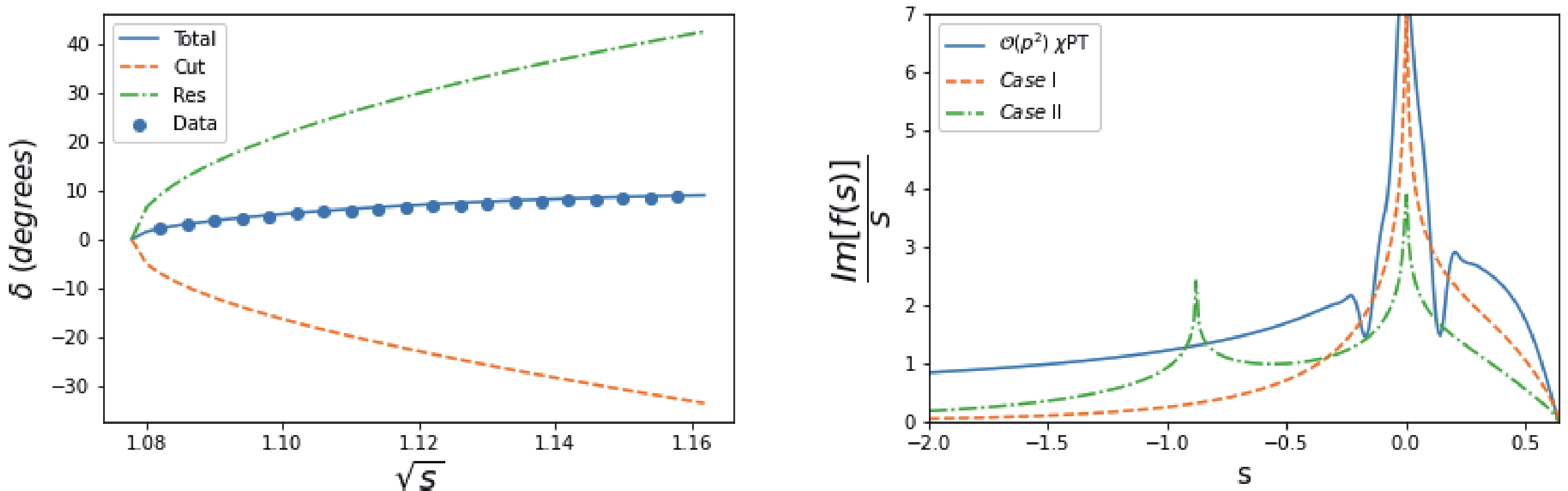
Figure 3. (color online) (left)
$ N/D $ fit to the$ S_{11} $ phase shift with$ \mathcal{O}(p^2) $ $ \chi $ PT input; (right) a comparison of different$ {\mathrm{Im}f(s)}/{s} $ in different situations.As a comparison, Fig. 3 plots the "spectral function," i.e.,
$ {\mathrm{Im}_Lf(s)}/{s} $ , obtained here, together with those discussed in Sec. II.B. Comparing Eq. (39) with that in Table 1 and the different$ l.h.c $ contributions in Fig. 3, we observe that the$ \mathcal{O}(p^2) $ calculation overestimates the$ l.h.c $ contribution, compared with that of$ Case $ II. As a result, the pole contribution to the phase shift must be increased, and the pole location moves towards to the right direction in the$ s $ plane, closer to the$ \pi N $ threshold. However, such discussions are only meaningful under the condition that the effects of the spurious branch cut and the spurious pole around$ s = \Lambda^2_R $ cancel each other out.If all the spurious contributions are ignored④, this presents a problem. The calculation here and that in Ref. [3] use the same "data" sample and
$ l.h.c. $ , while in Ref. [3], the pole locates at$ \sqrt{s} = 0.86\pm 0.05- {\rm i}(0.13\pm0.08) $ GeV. Compared to Eq. (39), there exists a rather large systematic error in determining the pole location. One possible reason may be that in Ref. [3] a truncation of$ l.h.c. $ is performed, while in this calculation, there is no truncation on the l.h.s; see Eq. (7). In fact, in the calculation in Table 4 of Ref. [3], it is found that when sending the cutoff$ s_c $ to$ \infty $ , the pole location moves upwards to$ \sqrt{s} = 0.91- {\rm i}0.21 $ GeV, i.e., closer to Eq. (39).Finally, we also tested the
$ \mathcal{O}(p^3) $ inputs (at tree level only) and found that the outputs are similar to the situation found in the$ \mathcal{O}(p^2) $ case; therefore, the results are not discussed in detail here. -
In the above section, we have discussed the problem encountered when using
$ \chi $ PT results to estimate the$ l.h.c $ . The higher order terms in the chiral lagrangian describing$ \pi $ N interactions are obtained by integrating out heavy degrees of freedom, such as the$ \rho $ meson in the$ t $ -channel and$ N^* $ resonances in the$ s $ and$ u $ -channels⑤. The problematic singularities at$ s = 0 $ in partial wave chiral amplitudes are at least partly a result of integrating out heavy degrees of freedom. To demonstrate this clearly, let us consider an effective interaction lagrangian, responsible for$ t $ -channel$ \rho $ meson exchange,$ \mathcal{L}_{t} = g_{\rho}\vec{\rho}^\mu\cdot(\partial_\mu \vec{\pi}\times \vec{\pi})+g_{\rho}\bar{N}\dfrac{1}{2}\vec\tau\cdot\left(\gamma^\mu\vec{\rho}_\mu+\dfrac{\kappa}{2m_N}\sigma^{\mu\nu}\partial_\mu\vec{\rho}_\nu\right)N\ , $

(40) where
$ g_{\rho} $ and$ \kappa $ are resonance coupling constants,$ \vec{\tau} $ are Pauli matrices, and$ \vec{\rho}_{\mu} $ ,$ \vec{\pi} $ , and$ N $ refer to$ \rho $ resonance, pion, and nucleon, respectively. For the$ S_{11} $ channel, the$ \rho $ exchange contribution to the invariant amplitude, Eq. (19), can be obtained:$ A = \frac{g_{\rho}^2\kappa(u-s)}{2m_N(t-m_{\rho}^2)}\ ,\quad B = \frac{2 g_{\rho}^{2}(\kappa+1)}{t-m_{\rho}^{2}}\ . $

(41) If a
$ 1/m_{\rho} $ expansion is performed at the leading order, we have$ A = \frac{g_{\rho}^{2} \kappa(s-u)}{2 m_{N} m_{\rho}^{2}}\ ,\quad B = -\frac{2 g_{\rho}^{2}(\kappa+1)}{m_{\rho}^{2}}\ . $

(42) Compared to Eq. (22), we find that the
$ \rho $ meson exchange only contributes to the$ c_4 $ term [29]. As we already know from the discussions in Sec. III.A, the$ c_4 $ term will cause an$ s^{-3/2} $ singularity following partial wave projection. This is avoidable, if we do not perform a$ 1/m_{\rho} $ expansion in the beginning. It can be seen that all the resonance exchange amplitudes contain the singularity of$ s^{-1/2} $ type at most when$ s = 0 $ . Therefore, partial wave projections and chiral expansions do not commute, which can be determined directly by evaluating the$ t $ -channel$ \rho $ exchange contributions, by performing partial wave projections of Eqs. (25) and (28).We perform an asymptotic expansion of the
$ \rho $ exchange contributions to$ T(S_{11}) $ in the vicinity of$ s = 0 $ and find that the two most singular terms are of type$ \frac{a+bs}{\sqrt{s}}\ ,$

(43) which are not of type
$ \mathcal{O}(s^{-5/2}) $ , which would be obtained if the$ \rho $ propagator were expanded beforehand. Similar results are found if we introduce, for example, a$ u $ -channel as well as an$ s $ -channel$ S_{11} $ resonance exchange.In this situation, it can be proven that expanding the
$ N^* $ propagator in the full amplitudes presents contributions to the$ c_3 $ and$ c_4 $ terms in Eq. (22). Avoiding a chiral expansion beforehand, the resonance exchange contribution to the partial wave amplitude can be expanded at$ s = 0 $ . Similar results to Eq. (43) are again obtained, for the$ P_{11} $ resonance exchange contributions.Explicit expressions for resonance contributions to parameters, e.g.,
$ a $ and$ b $ defined in Eq. (43), are obtainable. However, another significant problem occurs here. These coefficients depend on the mass parameters of the exchanged resonances and do not disappear as the resonance mass increases, which contradicts the general expectation from the decoupling theorem [30, 31]⑥. Without a deeper understanding of this problem, it should be noted that the sign of the contributions from different sources can be different. For example, the$ t $ -channel$ \rho $ exchange contribution to parameter$ a $ is$ a(\rho) = \rhbr -\dfrac{g_{\rho}^{2} \kappa\left(m_{N}^{2}-m_{\pi}^{2}\right)}{64 \pi m_{N}} $

the
$ \dfrac{1}{2}^{+} $ baryon exchange contribution is$ a(N^{*+}) = \dfrac{\left(g_{N^{*}}\right)^{2}\left(-m_{N}^{2}+m_{\pi}^{2}\right)\left(3 m_{N}^{2}+\left(m_{N^{*}}\right)^{2}\right)}{128 \pi F^{2} m_{N^{*}}} $

whereas the
$ \dfrac{1}{2}^{-} $ resonance exchange contribution is$ a(N^{*-}) = \dfrac{\left(g_{N^{*}}\right)^{2}\left(m_{N}^{2}-m_{\pi}^{2}\right)\left(3 m_{N}^{2}+\left(m_{N^{*}}\right)^{2}\right)}{128 \pi F^{2} m_{N^{*}}} $

which is different in sign from that of the first two contributions. Hence, a conspiracy theory of cancellation is assumed to overcome the problem of large resonance contributions to the parameter
$ a $ , or more accurately,$ T(s) $ near$ s = 0 $ . In practice, we therefore use the$ \mathcal{O}(p^1) $ $ \chi $ PT result plus a polynomial background as the input$ \mathrm{Im}_LT $ , i.e.,$ \mathrm{Im}_LT(s) = \mathrm{Im}_LT^{(1)}(s) + \mathrm{Im}_L\left[\dfrac{a+bs}{\sqrt{s}}\right]\ , $

(44) where
$ a $ and$ b $ are simply two free parameters, unrelated to resonance parameters. The fit gives$ N(s_0) = 0.57 $ ,$ a = -2.39 $ GeV, and$ b = -6.27 $ GeV$ ^{-1} $ , and one second sheet pole is found with$ \sqrt{s} = 0.95- 0.25{\rm i} $ GeV without sizable spurious branch cut contributions.As the mass of the
$ \rho $ meson is fixed, we also explored the case of$ \mathcal{O}(p^1) $ $ \chi $ PT results plus the$ \rho $ meson exchange term and a polynomial. That is,$ \mathrm{disc}\,T(s) = \mathrm{disc}\,T^{(1)}(s) +\mathrm{disc}\,T^{\rho}(s)+ \mathrm{d\mathrm{\mathrm{}}isc}\,\left[\dfrac{a+bs}{\sqrt{s}}\right]\ . $

(45) In this case, the
$ \rho $ meson exchange produces an extra arc in the$ s $ plane [9]; see Fig. 4. We get$ {N(s_0) = 0.61,} $ $ a = -7.88 $ GeV, and$ b = -8.00 $ GeV$ ^{-1} $ , and one second sheet pole is found to be located at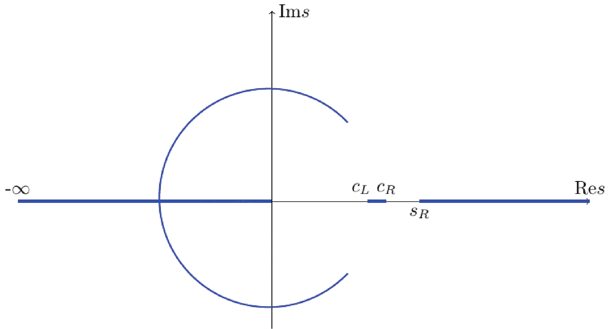
$ \sqrt{s} = 0.90- 0.20{\rm i}\; \mathrm{GeV}\ . $

(46) These solutions are not stable – there exists other solutions but with similar behaviours. In all cases, the contributions from the spurious branch cuts are negligible, compared with the results from the
$ {\cal O}(p^2) $ case, and the$ N^*(890) $ pole location remains stable. It is noticed that the contribution from the arc cut generated by$ t $ -channel$ \rho $ exchange is very small, e.g., it only contributes 1.5$ ^\circ $ at$ \sqrt{s} = 1.16 $ GeV.The "spectral" function in this case is plotted in Fig. 5. Different contributions to the phase shift according to the PKU decomposition are plotted in Fig. 6.
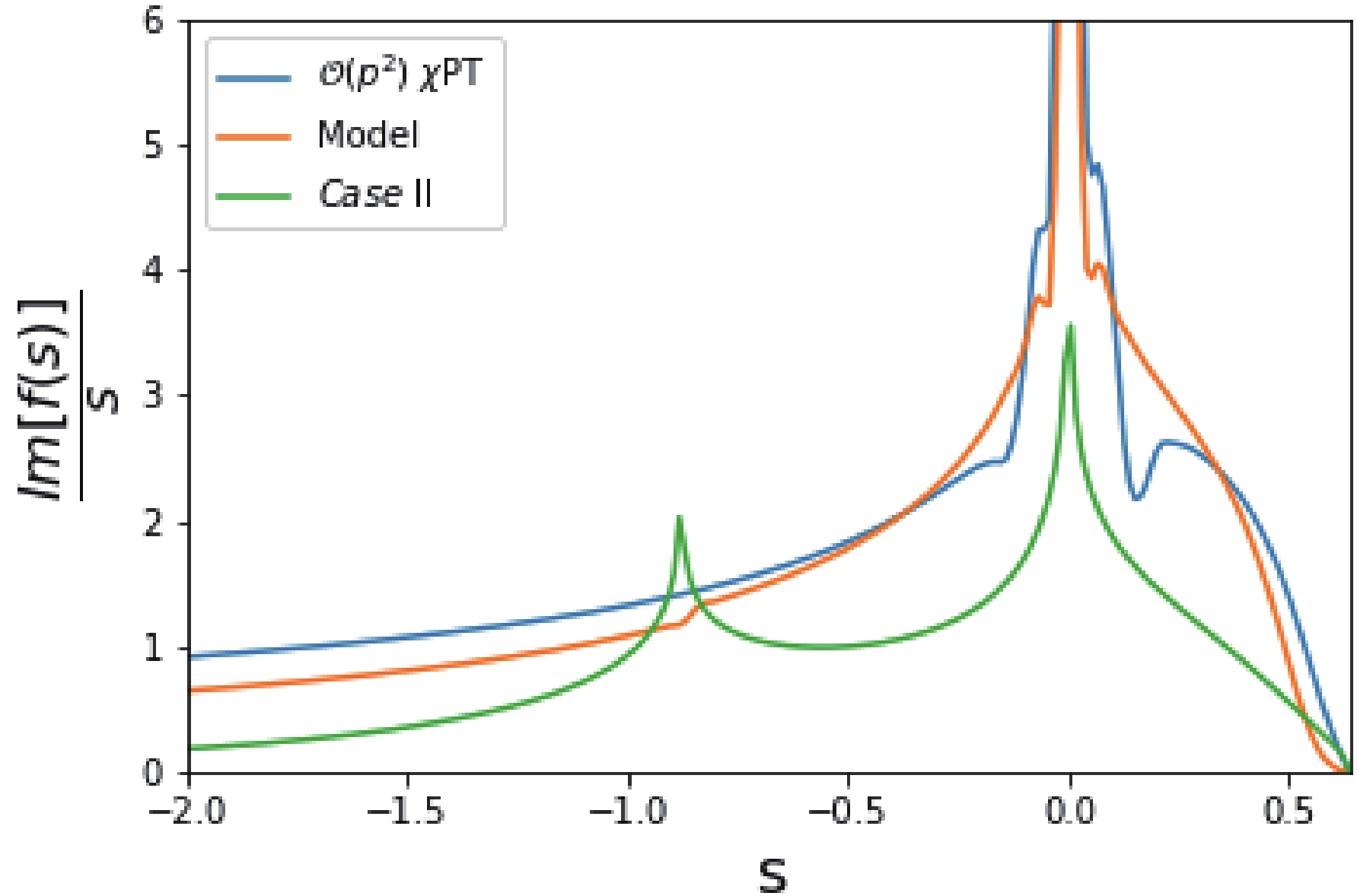
Figure 5. (color online) Comparison among different "spectral" functions. The singular behaviors of
$ T(s) $ at$ s = 0 $ are$ \mathcal{O}(s^{-5/2}) $ ,$ \mathcal{O}(s^{-1/2}) $ , and$ \mathcal{O}(s^{0}) $ for$ \mathcal{O}(p^2) $ $ \chi $ PT, model Eq. (45), and$ Case $ II, respectively.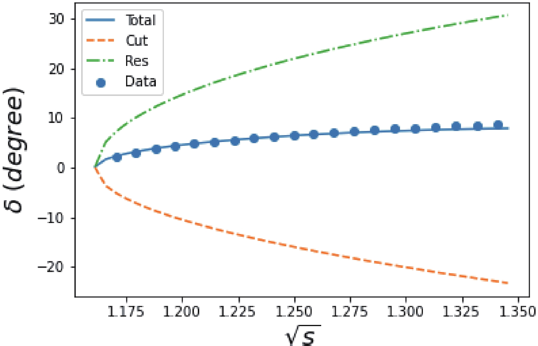
Figure 6. (color online) Fit results using Eq. (45). Phase shift decomposition: only contributions from physical components are plotted including their summation "Total." It clearly demonstrates that spurious contributions cancel each other out; otherwise, the curve "Total" cannot move closer to the data.
Before closing the discussions on the numerical calculations, it should be stressed that the major physical outputs have limited reliance on the choice of the cutoff parameter
$ \Lambda_R^2 = 1.48 $ GeV$ ^2 $ . For example, setting$ \Lambda_R^2 = 2.0,2.5 $ GeV$ ^2 $ in model Eq. (45) results in almost the same pole location at$ \sqrt{s} = 0.897-{\rm i}0.193 $ GeV.In the previous sections, we have presented extensive and thorough analyses. However, there are inherent limitations to the work that present avenues for further analyses, which could be explored in future studies. All the calculations in this paper are performed at the tree level only. At the loop level, there are certainly dynamical cut contributions, such as the circular cut. The latter is estimated in Ref. [1] using the complete
$ \mathcal{O}(p^3) $ $ \chi $ PT input, and it is found that the sign of the circular cut contribution may vary depending on the choice of cutoff parameter but always remains small in magnitude, e.g., at$ \sqrt{s} = 1.16 $ GeV its contribution to the phase shift is 0.2$ ^\circ $ when$ s_c = 0.32 $ GeV$ ^2 $ , and –1.7$ ^\circ $ when$ s_c = -0.08 $ GeV$ ^2 $ . When evaluating the circle, the problematic situation of$ s = 0 $ is not present; therefore, we believe that this estimation of the size of the circular cut contribution is at least qualitatively reasonable. From Fig. 7, the cutoff parameter$ s_c = 0.32 $ GeV$ ^2 $ corresponds to evaluating the$ l.h.c. $ region covered by the green dashed circle, which can be estimated by chiral perturbation theory; whereas$ s_c = -0.08 $ GeV$ ^2 $ corresponds to the region covered by the red dotted circle, which is required by the best fit. The estimations made in Refs. [1, 3] determined that the region where the$ \chi $ PT calculation can be safely used is not suffcient to generate$ N^*(890) $ ⑦, i.e., help from the contribution in the region$ s\in(-\infty, 0.32) $ is needed⑧. The singularity in the "spectral" function at$ s = 0 $ seems to be helpful. It is realized that the rescue task is easily fulfilled by examining Fig. 5. The fit Case II only contains a weak singularity at$ s = 0 $ , i.e.,$ T(0)\propto \mathrm{const} $ , while its contribution in the segment$ (0.32, s_L] $ is much weaker than those of$ \mathcal{O}(p^2) $ but still affords a pole. The real situation should be much more optimistic. It is noticed that the model Eq. (44) behaves similar to the$ \mathcal{O}(p^2) $ $ \chi $ PT results in the region$ (0.32, s_L) $ , and it is expected to continue operating in the region$ (-\Lambda^2_L, -\epsilon)\cup(+\epsilon, 0.32) $ , where$ \Lambda^2_L $ is estimated to be approximately$ R = m_N^2-m_\pi^2 $ for example. We create a test by setting$ \epsilon\simeq 0.05 $ GeV$ ^2 $ and cut off the peak around$ s = 0 $ in the "spectral" function, when$ s\in(-\epsilon, +\epsilon) $ .$ N^*(890) $ emerges with a location$ \sqrt{s} = 0.89-0.24{\rm i} $ GeV.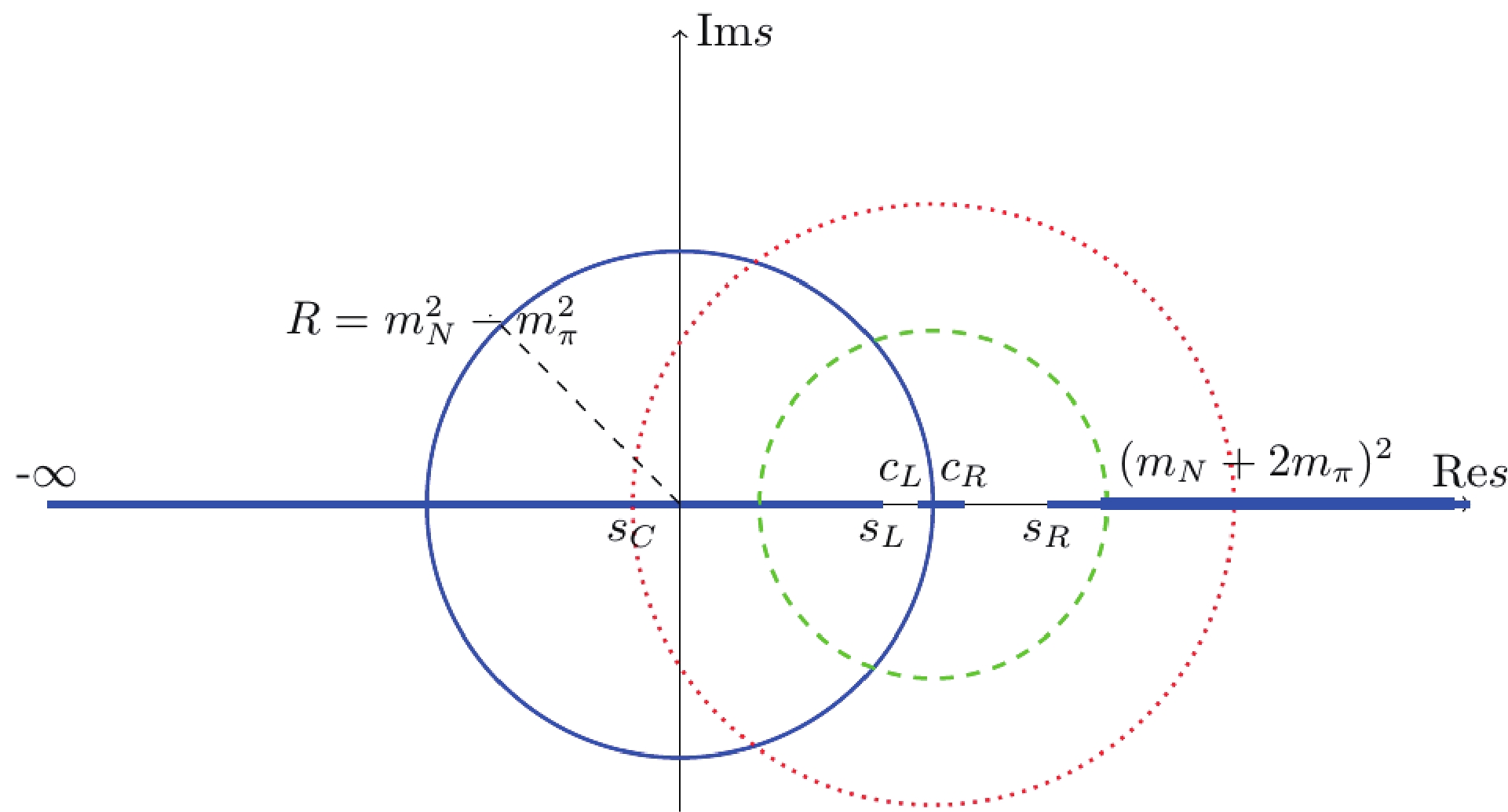
Figure 7. (color online) Region of
$ l.h.c. $ used in Ref. [1]. The cutoff parameter$ s_c = 0.32 $ GeV$ ^2 $ corresponds to evaluating the$ l.h.c. $ region covered by the green dashed circle, which can be estimated by the chiral perturbation theory, whereas$ s_c = -0.08 $ GeV$ ^2 $ corresponds to the region covered by the red dotted circle, which is required by the best fit.Hence, we conclude that the
$ l.h.c. $ contributions in total to the phase shift are sizable, based on which,$ N^*(890) $ survives with a rather stable pole location. Considering the level of accuracy of our calculations, statistical error bars are not presented in this paper. -
It may be bold to claim a new discovery in a field that has been studied extensively for more than half a century. However, according to our studies, a subthreshold broad resonance exists if the
$ s $ -wave phase shift steadily rises above the threshold as a convex curve. The discussion presented in the previous section suggests that the kinematical singularity structure at$ s = 0 $ plays a rather important role. This is not surprising. In extreme cases, there are even examples where a pole can be generated for purely kinematic reasons. For example, in the$ J = 0,I = 2 $ channel of$ \pi\pi $ scatterings, there exists a virtual pole which can be understood through purely kinematical reasons, which presents important contributions to the phase shift [6] and can be proven to exist through rigorous testing [32]. Another example is the companionate virtual state of the nucleon, which can also be explained through purely kinematical reasons [3].It is also interesting to notice that the
$ N^*(890) $ state may be related to the lowest lying$ 1/2^- $ baryon states, first suggested by Azimov in 1970 [33] and named as$ N^\prime $ , having been the focus of many studies thereafter [34]. Contrary to the original proposal that the lowest lying nucleon counterparts lie above the$ \pi N $ threshold, or at least lie above the nucleon mass (on the first sheet), the pole position named$ N^*(890) $ determined in Refs. [1-3] as well as in this paper escapes all previously defined bounds and limits [34]. The mass (width) difference may be explained by a familiar mechanism that when a strong coupling is gradually formed, the pole will move from the real axis above the threshold to the left of the$ s $ plane, off the real axis. Nevertheless, it may also be possible for the$ N^*(890) $ "resonance" to be a virtual pole on the$ k $ plane, as suggested in Ref. [3]. In the latter situation, the "width" of$ N^*(890) $ does not need to have any relations with particle decays. There remains a significant avenue of work in identifying$ N^\prime $ and$ N^*(890) $ , to be explored in future studies.The
$ N/D $ calculations discussed in this paper are of a complex dynamical form. However, the production representation has been shown to be useful in providing a simple and pictorial way of understanding the essence of the$ N/D $ calculations: the evidence for the existence of$ N^*(890) $ seems to be partly from the peculiar singularity structure of the background integral, defined in Eq. (10). If$ T(s = 0) $ does not disappear (or does not disappear fast enough), then an$ s $ -wave subthreshold resonance exists, in the most attractive channels⑨. This may even be a universal phenomenon, if the background contributions are universally negative, as suggested by quantum scattering theory [36] and repeatedly verified by calculations in quantum field theories. [4, 6, 7]It is apparent that the existence of a light
$ 1/2^- $ nucleon state is crucial for the completion and establishment of the lowest lying$ 1/2^- $ octet baryons, as suggested in Ref. [33], should it exist⑩. This will significantly improve our understanding of strong interaction physics. For example, the$ N^*(890) $ state, should it exist, will force us to rethink the possible physics behind$ f_0(500) $ and$ K(700) $ . Another question raised is how to interpret the breaking of spontaneous chiral symmetry. The textbook explanation on this point is that the axial charge$ Q_A $ commutes with the strong interaction hamiltonian, hence, if chiral symmetry were not broken then parity doublets would appear in nature. However, the lowest lying$ 1/2^- $ nucleon observed is$ N^*(1535) $ and the non-degeneracy of its mass, compared with the nucleon mass, therefore indicates that chiral symmetry is spontaneously broken. The emergence of$ N^*(890) $ may also bring about a new way of thinking about the related physics.Finally, it is also determined in this paper that there exists two virtual poles located on the real axis, outside but very close to the
$ u $ channel cut$ [c_L, c_R] $ . Their existence is proven relying on the validity of chiral expansions up to all orders. -
The authors would like to thank Zhi-hui Guo and De-Liang Yao for helpful discussions at various stages of this work, and Ulf-G. Meißner for careful reading of the manuscript and useful suggestions. We especially thank Igor Strakovsky at George Washington University, for providing very useful information on the
$ 1/2^- $ octet baryons. -
The
$ u $ channel nucleon pole exchange diagram will contribute to the partial wave amplitude cut$ \in[c_L,c_R] $ , with$ c_L = {(m_N^2-m_\pi^2)^2}/{m_N^2} $ and$ c_R = m_N^2+2m_\pi^2 $ . The point$ s = c_L $ is reached when$ z_s = -1 $ and$ u = m_N^2 $ , and$ s = c_R $ is reached when$ z_s = +1 $ and$ u = m_N^2 $ (see Eq. (27)). More precisely, at branch points$ c_L $ and$ c_R $ , the leading term of the partial wave amplitude is determined by$ \begin{aligned}[b] & {s\to {c_L}:}\,\,\,T(s)\to -\frac{g^2 m_N^4 }{16 \pi F^2 \left(4 m_N^2-m_\pi^2\right)}\ln \frac{s-c_L}{c_L-c_R}\ ,\\ & {s\to {c_R}:}\,\,\,T(s)\to\frac{g^2 m_N^2 (m_N^2+2 m_\pi^2)} {\pi F^2 (4 m_N^2-m_\pi^2)}\ln \frac{c_R-c_L}{s-c_R}\ , \end{aligned} \tag{A1}$

which are solely from the
$ u $ channel nucleon pole term and are hence exact, i.e., receiving no chiral corrections. Based on Eq. (47),$ \begin{aligned}[b]&s\to c_L, \quad S^{}\simeq A_{c_L}+B_{c_L}\ln\frac{s-c_L}{c_L-c_R}\ ,\\& s\to c_R, \quad S^{}\simeq A_{c_R}+B_{c_R}\ln\frac{s-c_R}{c_R-c_L}\ ,\end{aligned}\tag{A2} $

in which the coefficients read
$ \begin{aligned}[b]A_{c_L} =& A_{c_R} = 1+\frac{g^2 m_N m_\pi}{8 \pi F^2}+O\left(m_\pi^3\right)\ ,\\ B_{c_L} =& B_{c_R} = \frac{g^2 m_N m_\pi}{16 \pi F^2}+O\left(m_\pi^3\right)\ . \end{aligned}\tag{A3} $

These equations are obtained from the Born term calculations, where
$ A_{c_L} $ ($ B_{c_L} $ ) and$ A_{c_R} $ ($ B_{c_R} $ ) differ at the$ O(m_\pi^3) $ level. It is worth emphasizing that$ A_{c_L} $ and$ A_{c_R} $ may receive chiral corrections, but$ B_{c_L} $ and$ B_{c_R} $ do not, as the latter is related to the residue of the$ u $ channel nucleon pole.One important conclusion is that
$ S(c_L), S(c_R)\to -\infty $ which are exact (correct at least to any order of chiral expansions) and are immune to any loop corrections. It should be remembered that$ S = +1 $ at$ s_L $ and$ s_R $ by definition, and$ S(s) $ is real when$ s\in (s_L, c_L)\cup(c_R, s_R) $ . There must be two$ S $ matrix zeros: one below$ c_L $ and another above$ c_R $ , on the real axis⑪. Their locations (denoted by$ v_L $ and$ v_R $ ) are$ \begin{aligned}[b]v_L =& c_L-(c_R-c_L){\rm e}^{-A_{c_L}/B_{c_L}}\ ,\\ v_R =& c_R+(c_R-c_L){\rm e}^{-A_{c_R}/B_{c_R}}\ . \end{aligned}\tag{A4} $

Even more surprisingly, these two virtual poles in total make a large contribution to the phase shift, as they provide approximately
$ 50^\circ $ at$ \sqrt{s} = 1.16 $ GeV, which is not in agreement with the picture presented in Figs. 3 and 6. The solution to this apparent paradox is complex.In the derivation of the production representation, Eqs. (10) and (12), it is generally assumed that the branch cut singularity structures of
$ S^{{\rm cut}} $ ($ = \exp\{2{\rm i}\rho(s)f(s)\} $ ) and$ f(s) $ (or$ \ln{S^{\rm cut}} $ ) are the same. This is not always true: when$ S^{\rm cut} $ is real and negative at a certain point,$ \ln S^{\rm cut} $ must be discontinuous when the sign of the imaginary part of$ S^{\rm cut} $ changes. This situation is true in the present case. Recall that at the$ O(p^1) $ level,$ \begin{aligned}[b] T^{(1)} =& -\frac{g^2 \left(-2 m_N^2 m_\pi^2-m_N^2 s-m_\pi^2 s+s^2\right)}{32 \pi F^2 \left(s-m_N^2\right)}+\frac{-m_N^2-m_\pi^2+s}{32 \pi F^2}\\ &+\frac{m_N \left(-m_N^2+m_\pi^2+s\right)}{32 \pi F^2\sqrt{s}}\\&-\frac{g^2 m_N \left(-m_N^4+m_N^2 m_\pi^2+m_N^2 s+2 m_\pi^2 s\right)}{32 \pi F^2 \left(s-m_N^2\right)\sqrt{s}}\\& +\frac{g^2 m_N^2 s^2 \left(-m_N^2-m_\pi^2+s\right)}{16 \pi F^2 \left(s-c_L\right)^2 \left(s-c_R\right)^2} \\&\times\left(\frac{m_N^2}{s}\left(s-c_L\right) \left(\log \frac{s-c_L}{s-c_R}+\log \frac{m_N^2}{s}\right)-s\rho(s)^2\right)\\ &-\frac{g^2 m_N^3 s^2 \left(-m_N^2+m_\pi^2+s\right)}{16 \pi F^2 \left(s-c_L\right)^2 \left(s-c_R\right)^2\sqrt{s}} \\&\times \left(\left(s-c_R\right) \left(\log \frac{s-c_L}{s-c_R}+\log \frac{m_N^2}{s}\right)-s\rho(s)^2\right)\ . \end{aligned} \tag{A5}$

It is determined from the above expressions that the cut
$ L\in (-\infty,0)\cup(c_L,c_R) $ . There are two sources contributing to the imaginary part of$ T(s) $ when$ s\in(-\infty,0) $ : one comes from the kinematical$ \sqrt{s} $ while another comes from the logarithmic function; when$ s\in(c_L,c_R) $ $ \mathrm{Im}T $ comes solely from the$ u $ channel nucleon pole exchange. On$ (c_L,c_R) $ , the imaginary part of$ T^{(1)} $ reads$ \begin{aligned}[b] \mathrm{Im}T^{(1)}(s) = &\frac{g^2 m_N^2 s^2 }{16F^2 \left(s-c_L\right)^2 \left(s-c_R\right)^2} \\ &\times\left[\dfrac{m_N^2}{s}(s-c_L)\left(-m_N^2-m_\pi^2+s\right)\right.\\&\left.-\dfrac{m_N}{\sqrt{s}}(s-c_R)\left(-m_N^2+m_\pi^2+s\right)\right]\ , \end{aligned} \tag{A6}$

from which it is determined that
$ \mathrm{Im}T^{(1)} $ develops a zero at$ s = s_c\simeq m_N^2-{m_\pi^4}/{2m_N^2} $ and changes sign when$ s $ crosses$ s_c $ . It is important to realize that Eq. (52) is immune to chiral perturbation corrections.From Fig. A1, it is found that the imaginary part of
$ S^{\rm cut} $ disappears at the point$ s_c $ , which is close to$ m_N^2 $ ; meanwhile, the real part of$ S^{\rm cut} $ is negative. In Fig. A1$ S^{\rm cut} $ is calculated by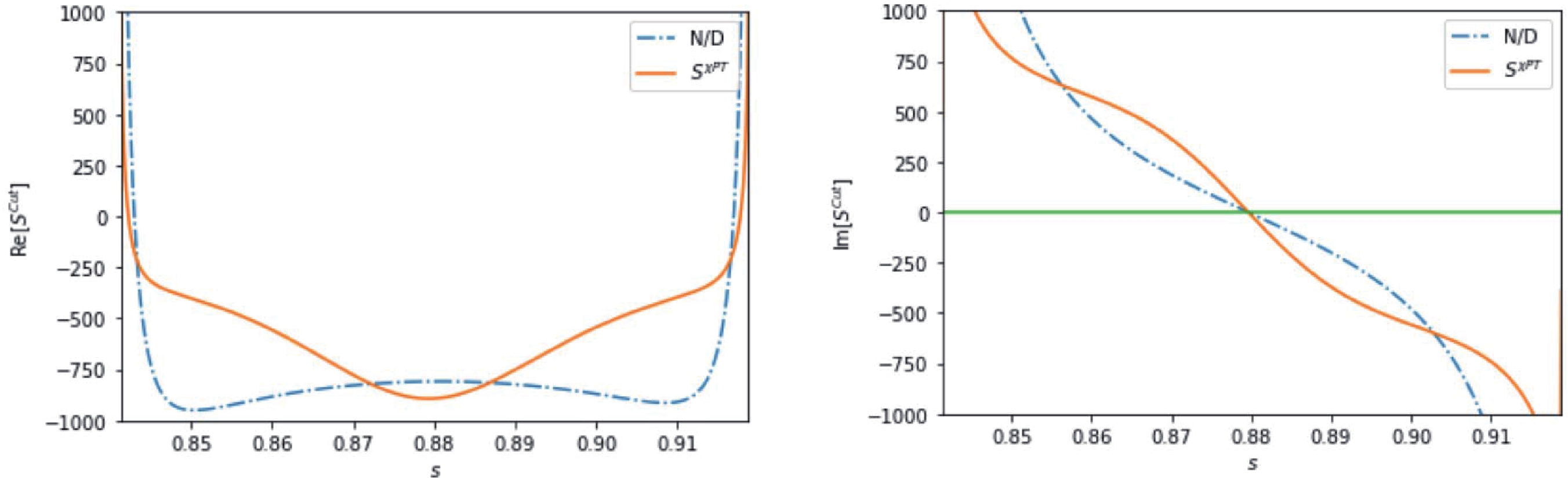
Figure A1. (color online) Real (left) and imaginary (right) parts of
$ S^{\rm cut}(s) $ when$ s $ lies in$ (c_L,c_R) $ . The dot-dashed line comes from the N/D solution of Eq. (44); the yellow solid line is obtained from the$ O(p^1) $ $ \chi $ PT results.$ S^{\rm cut} = {S^{\rm phys}\over\prod_p S^{p}\times S^{v_L}\times S^{v_R}} \tag{A7} $

where the newly found virtual poles are included, and
$ S^{\rm phys} $ is approximated by both the unitary amplitude obtained by fitting Eq. (44) and the pure$ O(p^1) $ perturbation amplitude⑫. From Fig. A1 , it is seen that at$ s = s_c $ ,$ \ln S^{\rm cut} $ must develop a discontinuity, and hence, a branch cut emerges crossing$ s_c $ . It is numerically verified that the cut is an arc on the complex$ s $ -plane in the$ N/D $ solutions. It should be emphasized here that this unexpected additional cut does not affect the$ S^{\rm cut} $ , as across the cut the discontinuity of$ \ln S^{\rm cut} $ is$ 2i\pi $ and has no influence on the value of an exponential. Though not producing any issues in the analyticity structure of$ S^{\rm cut} $ , the additional cut of$ \ln S^{\rm cut} $ , or the dispersive representation of the function$ f $ defined in Eq. (10), must be changed as the integration contour has to be modified.The problem determined above is significant as the distorted contour may depend on numerics, hence being impossible to control. However, it can be overcome by the following consideration. We define
$ \bar f(s) = \dfrac{\ln-S^{\rm cut}}{2{\rm i}\rho(s)}- \dfrac{\pi}{2\bar\rho(s)} \tag{A8}$

where the function
$ \bar\rho(s) $ is the "deformed"$ \rho(s) $ with its cut$ \in [s_L, s_R] $ , while the cut of the latter is defined as$ (-\infty, s_L]\cup [s_R,+\infty) $ . Notice that$ \bar \rho(s) $ and$ \rho(s) $ are identical in the physical region. The function$ \bar f(s) $ is identical to$ f(s) $ when$ s $ is also in the physical region but differs in the cut alignment. Particularly,$ \bar f $ no longer contains the arc cut of$ f $ , as$ s_c $ is no longer a branch point of$ \bar f $ . However,$ \bar f $ contains an additional cut induced by$ \bar\rho $ , which is absent in$ f $ . Both the terms on the$ r.h.s. $ of Eq. (54) contain cuts on$ [s_L,s_R] $ , but the two cuts cancel each other out when$ s\in [c_R,s_R] $ . Hence, the left cut of$ \bar f $ on the real axis is actually$ [-\infty, c_R] $ , compared with the left cut of$ f $ on the real axis:$ [-\infty, s_L]\cup[c_L,c_R] $ . The dispersive integral representation of$ \bar f $ can be written as$ \begin{aligned}[b]\bar f(s) =& \dfrac{s}{\pi}\int_L\dfrac{\mathrm{Im}[\ln {-S^{\rm cut}(s^\prime)}/(2{\rm i}\rho(s^\prime))]}{s^\prime(s^\prime-s)}{\rm d}s^\prime\\& {+\dfrac{s}{\pi}\int_{s_L}^{c_L}\dfrac{\mathrm{Im}[\ln {-S^{\rm cut}(s^\prime)}/(2{\rm i}\rho(s^\prime))]}{s^\prime(s^\prime-s)}{\rm d}s^\prime}\\& {-s\int_{s_L}^{c_R}\dfrac{\mathrm{Im}[1/(2\bar\rho(s^\prime))]}{s^\prime(s^\prime-s)}{\rm d}s^\prime}\ . \end{aligned}\tag{A9} $

In the first term on the
$ r.h.s. $ of the Eq. (A9), the integration domain$ L = (-\infty, s_L]\cup[c_L,c_R] $ , i.e., the same as that in Eq. (10). Actually, the first term is identical to$ f $ defined in Eq. (10), as in the integrand$ S^{\rm cut} $ can be replaced by$ S^{\rm phys} $ . To prove this, firstly, on$ (-\infty, s_L] $ ,$ \mathrm{Im}[\ln {-S^{\rm cut}}/(2{\rm i}\rho)] = -\ln {|S^{\rm cut}|}/(2\rho) $ , and$ |S^{\rm cut}| = |S^{\rm phys}| $ . Secondly, the integral on$ [c_L,c_R] $ can be recast as$ \begin{aligned}[b]&\dfrac{s}{\pi}\int_{c_L}^{c_R}\dfrac{\mathrm{Im}[\ln {-S^{\rm cut}(s^\prime)}/(2{\rm i}\rho(s^\prime))]}{s^\prime(s^\prime-s)}{\rm d}s^\prime \\=& \dfrac{s}{2{\rm i}\pi}\int_{c_L}^{c_R}\dfrac{\ln[S^{\rm cut}_+/S^{\rm cut}_-]}{2{\rm i}\rho(s^\prime)s^\prime(s^\prime-s) }{\rm d}s^\prime\\ =& \dfrac{s}{2{\rm i}\pi}\int_{c_L}^{c_R}\dfrac{\ln[S^{\rm phys}_+/S^{\rm phys}_-]}{2{\rm i}\rho(s^\prime)s^\prime(s^\prime-s) }{\rm d}s^\prime \\=& \dfrac{s}{\pi}\int_{c_L}^{c_R}\dfrac{\mathrm{Im}[\ln {S^{\rm phys}(s^\prime)}/(2{\rm i}\rho(s^\prime))]}{s^\prime(s^\prime-s)}{\rm d}s^\prime\ , \end{aligned}\tag{A10}$

where
$ S_{\pm}\equiv S(s\pm {\rm i}\epsilon) $ . Hence, we complete the proof.The second integral in Eq. (A9) is analytically integrable, once it is realized that
$ S^{\rm cut} $ is positive along$ [s_L, c_L] $ , and the third integral is also integrable. The sum of the two integrals provides a contribution to the phase shift that is exactly canceled by the contribution from the two virtual poles, when their positions are taken at$ c_L $ and$ c_R $ . If the two virtual pole locations are fixed by Eq. (A4), the net effects of the sum of virtual poles and the additional cut are very small (e.g., of order of$ {10^{-3}} $ degrees at$ \sqrt{s} = 1.16 $ GeV). Therefore, the calculation using Eq. (10) is still valid, with a high accuracy, when the existence of the two virtual poles is ignored. Further, it is worth emphasizing that after such a calculation, there no longer exists the unwanted cut in$ \ln S^{\rm cut} $ crossing$ s_c $ , as verified by numerical analyses. Moreover, it should be noted that in numerical analyses, there may appear additional cuts in$ \ln S^{\rm cut} $ as well on the$ s $ plane in the distance, which is caused by the peculiar analyticity property of the logarithmic function. However, it is simple to prove that it is not hazardous and can simply be ignored.The discussions in this appendix can also be extended to higher partial waves, providing interesting results, which will be presented in future studies.
An N/D study of the S11 channel πN scattering amplitude
- Received Date: 2021-08-03
- Available Online: 2022-02-15
Abstract: Extensive dynamical


 DownLoad: