


 Abstract
 HTML
HTML Reference
 Related
 PDF
PDF


-
Nonlinear systems endowed with a deterministic nature may behave in a complicated, highly unpredictable, and “chaotic” way. General relativity is a nonlinear dynamical theory, and chaotic behavior in general relativity has been extensively studied, such as in the chaoticity of cosmological solutions [1, 2]. Among various dynamical systems investigated in general relativity, the test motion in a given black hole spacetime is a popular topic in literature, since it is of astrophysical relevance and provides some important insights into AdS/CFT correspondence.
However, it is well known that the geodesic motion of a point particle in the generic Kerr-Newman black hole spacetime is fully integrable [3]. To induce chaos, one can resort to spacetimes with more complicated geometries, external potentials imposed on test bodies, perturbations introduced to backgrounds, or test bodies endowed with internal structure. For a point particle, chaotic behavior of the geodesic motion has been investigated in several static axisymmetric spacetimes [4], multi-black hole spacetimes [5], bumpy spacetimes [6], weakly magnetized Schwarzschild black holes [7], black holes with discs or rings [8], the Schwarzschild-Melvin black holes [9], accelerating black holes [10] and spacetimes with a quadrupole mass moment [11]. In a universal way, the particle chaotic motion has lately been studied near the black hole horizon [12-14]. Interestingly, gravitational waves emitted from chaotic motions of particles in a bumpy spacetime can be used to distinguish an extreme-mass-ratio inspiral into a Kerr background spacetime from one into a non-Kerr background spacetime [15]. Recently, it has been shown that such a proposal may be undermined due to chaos suppression by frame dragging [16]. Partly motivated by AdS/CFT correspondence, the chaotic dynamics of a ring string have been studied in various black hole backgrounds [17-22] since the geodesic motion of a ring string was shown to exhibit chaotic behavior in a Schwarzschild black hole [23]. In addition, as a simplified model describing extreme mass ratio inspirals, the motion of a spinning test particle in black hole backgrounds was considered and also demonstrated to possess some chaotic features [24-27].
In contrast, the existence of a minimal measurable length has been predicted in various quantum theories of gravity such as string theory [28-32]. To incorporate the minimal length into quantum mechanics, the Heisenberg uncertainty principle can be modified, giving the so called "generalized uncertainty principle (GUP)" [33, 34]. Usually, the fundamental commutation relation is deformed to realize the GUP. For a 1D quantum system, the deformed commutator between position and momentum can take the following form
$ \lbrack X,P] = {\rm i}\hbar(1+\beta P^{2}), $

(1) where
$ \beta $ is some deformation parameter, and the minimal length is$ \Delta X_{\min} = \hbar\sqrt{\beta} $ . Many minimal length deformed quantum systems have been investigated intensively in literature, e.g., the harmonic oscillator [35], Coulomb potential [36, 37], gravitational well [38, 39], quantum optics [40, 41], compact stars [42-44], and cosmology [45-47]. Furthermore, taking the classical limit$ \hbar\rightarrow0 $ , one can discuss the minimal length effects on classical systems, such as observational tests of general relativity [48-55], classical harmonic oscillator [56, 57], equivalence principle [58], Newtonian potential [59], the Schrödinger-Newton equation [60], the weak cosmic censorship conjecture [61], and motions of particles near a black hole horizon [62-64]. In addition, the minimal length corrected Hawking temperature can be obtained by using the Hamilton-Jacobi method [65-69].In this paper, we discuss the minimal length effects on the motion of a particle under a harmonic potential in the Rindler space, which is the approximation of the near-horizon region. This study is a follow-up of our previous works [62, 70], which demonstrated that the minimal length effects tend to increase chaos. Analytical approaches, i.e., the perturbation method and Melnikov method, were employed to investigate the chaotic motion of a particle around a black hole in [62, 70]. Here, we numerically study the motion of a particle and the corresponding chaos indicators in the Rindler space. Our numerical results not only support the findings of [62, 70] but also signal a shorter scrambling time, a notion that is connected to chaos.
The rest of this paper is organized as follows. In section II, we obtain the equations of motion for the dynamical system. The dynamics of the system are numerically analyzed in section III. We summarize our results with a brief discussion in section IV. In this paper, we take Geometrized units
$ c = G = k_{\rm B} = 1 $ , where the Planck constant$ \hbar $ is the square of the Planck length$ \ell_{\rm p} $ . -
To study the minimal length effects on the chaotic dynamics of a particle, we consider the motion of the particle in the near-horizon region, where chaotic behavior can be induced. Specifically, we discuss a relativistic particle moving in the near-horizon region of a 4D spherically symmetric black hole with the metric
$ {\rm d}s^{2} = -h\left( r\right) {\rm d}t^{2}+\frac{{\rm d}r^{2}}{g\left( r\right) } +r^{2}\left( {\rm d}\theta^{2}+\sin^{2}\theta {\rm d}\phi^{2}\right) , $

(2) where
$ h\left( r\right) $ and$ g\left( r\right) $ are assumed to have a simple zero at the event horizon$ r = r_{+} $ . By the analytic continuation to Euclidean signature$ \tau = {\rm i}t $ , the above metric becomes$ {\rm d}s_{E}^{2} = h\left( r\right) {\rm d}\tau^{2}+\frac{{\rm d}r^{2}}{g\left( r\right) }+\cdots. $

(3) Near the horizon, one can approximate
$\begin{aligned}[b] {\rm d}s_{E}^{2} =& h^{\prime}\left( r_{+}\right) \left( r-r_{+}\right) {\rm d}\tau ^{2}+\frac{{\rm d}r^{2}}{g^{\prime}\left( r_{+}\right) \left( r-r_{+}\right) }+\cdots \\=& {\rm d}\rho^{2}+\rho^{2}{\rm d}\left( \frac{\sqrt{h^{\prime}\left( r_{+}\right) g^{\prime}\left( r_{+}\right) }}{2}\tau\right) ^{2}+\cdots, \end{aligned}$

(4) where we introduced a new coordinate
$ \rho\equiv2\sqrt{\left( r-r_{+}\right) /g^{\prime}\left( r_{+}\right) } $ . To evade a conical singularity at$ \rho = 0 $ , it is necessary to impose a periodicity$ \beta = 4\pi/\sqrt{h^{\prime}\left( r_{+}\right) g^{\prime }\left( r_{+}\right) } $ in the Euclidean time$ \tau $ . From thermal quantum field theory, the Hawking temperature of the black hole is given by$ \hbar/\beta $ . Therefore, the Hawking temperature is$ T = \frac{\hbar\sqrt{g^{\prime}\left( r_{+}\right) h^{\prime}\left( r_{+}\right) }}{4\pi}\equiv\frac{\hbar\alpha}{2\pi}, $

(5) where we define the surface gravity
$ \alpha\equiv\sqrt{g^{\prime}\left( r_{+}\right) h^{\prime}\left( r_{+}\right) }/2 $ for later use. To explore the region near the horizon, we introduce the proper distance from the horizon,$ x = \int_{r_{+}}^{r}\frac{{\rm d}r}{\sqrt{g\left( r\right) }}\sim\frac {2\sqrt{r-r_{+}}}{\sqrt{g^{\prime}\left( r_{+}\right) }}, $

(6) which measures the physical distance along radial direction (i.e.,
$ {\rm d}t = {\rm d}\theta = {\rm d}\phi = 0 $ ) from the horizon since$ {\rm d}x^{2} = {\rm d}r^{2}/g\left( r\right) $ . If one focuses on a small angular near-horizon region centered at$ \theta = 0 $ , the near-horizon metric of the black hole can be rewritten in terms of x:$ {\rm d}s^{2} = -\alpha^{2}x^{2}{\rm d}t^{2}+{\rm d}x^{2}+{\rm d}y^{2}+{\rm d}z^{2}, $

(7) where we introduce Cartesian coordinates,
$ y = r_{+}\theta\cos\phi,\;\;\;\;\;\;\;\;z = r_{+}\theta\sin\phi. $

(8) The metric
$ \left( 7\right) $ is the Rindler space, which describes the near-horizon geometry of the black hole$ \left( 2\right) $ . Note that the black hole horizon is at$ x = 0 $ in the Rindler coordinates. Since we are interested in the motion of a particle in the near-horizon region, we confine ourselves here to considering the Rindler space.It is well known that the geodesic equation in the metric
$ \left( 2\right) $ is separable; hence, the geodesic motion of a particle is integrable. To make the motion of a particle chaotic, one can impose an external potential outside the horizon. In what follows, we assume that the potential is a harmonic potential centered at$ (x,y,z) = (x_{0},0,0) $ with$ x_{0}>0 $ ,$ V\left( x,y,z\right) = \frac{\omega^{2}}{2}\left[ \left( x-x_{0}\right) ^{2}+y^{2}+z^{2}\right] , $

(9) where
$ \omega $ is the angular frequency. Practically, for any external potential, when a particle is displaced slightly from its stable equilibrium position, we can approximate the external potential by the harmonic potential. Therefore, our analysis with a harmonic potential in Rindler space can illustrate the motion of a particle near stable equilibrium, which is close to the horizon. For example, in an extreme-mass-ratio black hole binary system, Lagrange equilibrium points (where a particle is in equilibrium) can be close to the horizon of the light black hole due to the extreme mass ratio of the two black holes. In addition to the possible relation to astrophysics, the harmonic potential is of further academic interest as it may be used as a simple external potential for studying chaotic motion near the horizon. In this instructive toy model, the system is integrable with the absence of gravity, and hence, observing chaotic behavior due to gravity or quantum gravity effects will be easier. In [12, 71], the near-horizon chaotic motion of a particle under the harmonic potential was considered in the context of general relativity without quantum gravity effects.In the framework of usual non-relativistic quantum mechanics, a system is described by a state vector, and the dynamics is governed by the Schrödinger equation. In the classical regime with
$ \hbar\rightarrow 0 $ , the state vector becomes represented by a trajectory in phase space obeying Hamilton's equation (or equivalently, the corresponding Hamilton-Jacobi equation). In the classical limit$ \hbar\rightarrow 0 $ , the Heisenberg uncertainty principle becomes$ \Delta X\Delta P\geqslant\frac{\hbar}{2}\rightarrow0, $

(10) and hence, the position and momentum can be determined simultaneously, which is essential for defining a trajectory. For deformed quantum mechanics with the deformed commutator
$ \left( 1\right) $ , the corresponding generalized uncertainty principle is given by$ \Delta X\Delta P\geqslant\frac{\hbar}{2}[1+\beta(\Delta P)^{2}], $

(11) where the lower bound also goes to zero as
$ \hbar\rightarrow 0 $ . In the classical limit$ \hbar\rightarrow0 $ of deformed quantum mechanics, one can also determine the position and momentum simultaneously and associate a trajectory to a wave function. Therefore, it is proper to use the deformed Hamilton-Jacobi equation, which is derived from deformed quantum mechanics in the classical limit, to study the minimal length effects on a trajectory in the classical regime.Incorporating the deformed fundamental commutation relation
$ \left( 1\right) $ , the minimal length deformed Hamilton-Jacobi equation for the motion of a particle under an external potential has been derived in [62]. To be self-contained, we give the derivation of the deformed Hamilton-Jacobi equation in the appendix. In the Rindler space with the harmonic potential$ V\left( x,y,z\right) $ , the deformed Hamilton-Jacobi equation then becomes$ \frac{1}{\alpha^{2}x^{2}}\left[ \frac{\partial S}{\partial t}+V\left( x,y,z\right) \right] ^{2}-{\cal{X}}\left( 1+\beta{\cal{X}}\right) ^{2} = m^{2}, $

(12) where
$ {\cal{X}}\equiv\left( \partial_{x}S\right) ^{2}+\left( \partial_{y}S\right) ^{2}+\left( \partial_{z}S\right) ^{2} $ , and S is the classical action. The first derivatives of S with respect to the spatial coordinates are the conjugate momenta,$ p_{i} = \frac{\partial S}{\partial x_{i}}\;\;\;\;\;\;(i = x,y,z), $

(13) and the Hamiltonian of the system corresponds to the first derivative of S with respect to the time,
$ {\cal{H}} = -\frac{\partial S}{\partial t}. $

(14) Solving the Hamilton-Jacobi equation
$ \left( 12\right) $ for$ {\cal{H}} $ gives the Hamiltonian$ {\cal{H}} = \alpha x\sqrt{p^{2}\left( 1+\beta p^{2}\right) ^{2}+m^{2} }+V\left( x,y,z\right) , $

where we define
$ p^{2}\equiv p_{x}^{2}+p_{y}^{2}+p_{z}^{2}. $

(15) The equations of motion for
$ x_{i} $ are$ \dot{x}_{i} = \frac{\partial{\cal{H}}}{\partial p_{i}} = \alpha xp_{i} \frac{\left( 1+\beta p^{2}\right) \left( 1+3\beta p^{2}\right) } {\sqrt{p^{2}\left( 1+\beta p^{2}\right) ^{2}+m^{2}}}\;\;\;\;\;(i = x,y,z), $

(16) and those for
$ p_{i} $ are$ \begin{aligned}[b] \dot{p}_{x} =& -\frac{\partial{\cal{H}}}{\partial x} = -\alpha\sqrt {p^{2}\left( 1+\beta p^{2}\right) ^{2}+m^{2}}-\omega^{2}\left( x-x_{0}\right) ,\\ \dot{p}_{y} =& -\frac{\partial{\cal{H}}}{\partial y} = -\omega^{2}y{, }\dot{p}_{z} = -\frac{\partial{\cal{H}}}{\partial z} = -\omega^{2}z{.} \end{aligned} $

(17) The equations of motion for z and
$ p_{z} $ show that a particle that starts in the$ z = 0 $ plane remains in the$ z = 0 $ plane. For simplicity, we only consider the motion of a particle on the$ z = 0 $ plane in this paper. Therefore, we set$ z = 0 = p_{z} $ in the remainder of the paper. -
In this section, we study the dynamics of a particle moving in the Rindler space under the external potential
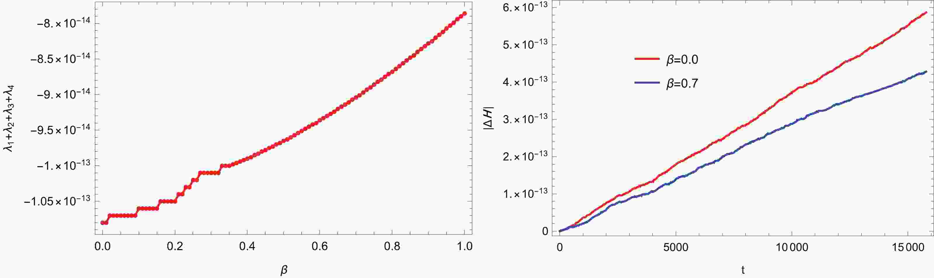
$ V\left( x,y,z\right) $ , with particular consideration of the minimal length effects on the chaotic dynamics. To detect chaotic phenomenon in the dynamical system, we resort to Poincaré surfaces of section and Lyapunov characteristic exponents (LCEs), which are calculated numerically. Since the chaotic motion of a particle is very sensitive to initial values, a numerical method with high precision is highly desirable. Here, we adopt Verner's "most efficient" Runge-Kutta$ 9(8) $ method [72], which can achieve high accuracy solving (with tolerances of$ <10^{-12} $ ). To test the accuracy of the numerical method, we consider two conserved quantities, namely the energy of the system E, which is conserved since there is no dissipation, and the sum of all LCEs$ \sum\nolimits_{i = 1}^{4}\lambda_{i} $ , which must be zero since a volume element of the phase space will stay the same along a trajectory for the conservative system. The left panel of Fig. 1 shows the sum of all LCEs as a function of$ \beta $ with the energy$ E = 5.0 $ . We also display the error of the energy$ \Delta{\cal{H}}\equiv {\cal{H}}\left( t\right) $ $ -{\cal{H}}\left( 0\right) $ along two trajectories with$ \beta = 0 $ and$ 0.7 $ , respectively, in the right panel of Fig. 1. It is demonstrated that the numerical method used in this paper can maintain the numerical error around or below$ 10^{-13} $ . We choose$ \alpha = 1 $ ,$ \omega = 10 $ ,$ m = 1 $ , and$ x_{0} = 1 $ for the numerical analysis in this section.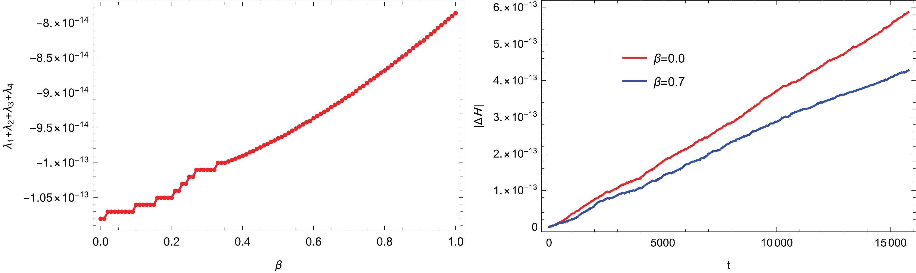
Figure 1. (color online) Numerical accuracy. (left) Sum of LCEs as a function of
$ \beta $ for$ E = 5.0 $ . (right) Errors of energy according to time for$ \beta = 0 $ and$ 0.7 $ . -
Invariant sets, such as fixed points and limit cycles, represent an important concept for understanding late time dynamics and the stability of a dynamical system. Here, in particular, we find the fixed point in the phase space of the dynamical system described by Eqs.
$ \left( 16\right) $ and$ \left( 17\right) $ and discuss the behavior near the corresponding fixed point. The fixed point in the phase space is determined by$ \dot {x}_{i} = 0 = \dot{p}_{i} $ , which leads to the fixed point solution$ x_{f} = x_{0}-\frac{m\alpha}{\omega^{2}}{,\;\;\;\;\; }y_{f} = 0{,\;\;\;\;\; }p_{xf} = 0,\;\;\;\;\;p_{yf} = 0. $

(18) Since
$ x_{f}\geqslant 0 $ in the Rindler space, the fixed point disappears when$ x_{0}< $ $ m\alpha/\omega^{2} $ . It is noteworthy that the equilibrium point of the system is also given by$ \dot{x}_{i} = 0 = \dot{p}_{i} $ . Therefore, the equilibrium point is$ x_{e} = x_{0}-\frac{m\alpha}{\omega^{2}},\;\;\;\;\;\;\;y_{e} = 0, $

(19) where
$ m\alpha/\omega^{2} $ is the displacement from the center of the harmonic potential due to the gravitational pull exerted on the particle. Near the fixed point, the nonlinear system can be approximated by a linear system represented by the Jacobian matrix, the eigenvalues of which determine the near-fixed point behavior. The eigenvalues of the Jacobian matrix at the fixed point$ \left( 18\right) $ are given by$ \left\{ {\rm i}\omega\sqrt{\frac{x_{f}\alpha}{m}},{\rm i}\omega\sqrt{\frac{x_{f}\alpha }{m}},-{\rm i}\omega\sqrt{\frac{x_{f}\alpha}{m}},-{\rm i}\omega\sqrt{\frac{x_{f}\alpha} {m}}\right\} . $

(20) Since the eigenvalues are purely imaginary, this fixed point is a center in the sense that trajectories near the fixed point are almost closed loops.
The fixed point solution
$ \left( 18\right) $ corresponds to the minimum energy of the system,$ E_{\min} = m\alpha x_{0}\left( 1-\dfrac {ma}{2\omega^{2}x_{0}}\right) $ . At the event horizon located at$ x = 0 $ , the energy of the system E should satisfy$ E\geqslant E_{\max}\equiv V\left( 0,0,0\right) = \frac{\omega^{2}x_{0}^{2}}{2}. $

Hence, for
$ E_{\min}<E<E_{\max} $ , the system wanders around the fixed point and can never reach or cross the event horizon. In Fig. 2, we present the orbits of the system in the x-y plane with the initial values$ E = 5.0 $ ($ >E_{\min} = 0.995 $ ),$ x\left( 0\right) = 0.99 $ ,$ p_{x}\left( 0\right) = 0.1 $ , and$ y\left( 0\right) = 0 $ for$ \beta = 0 $ ,$ 0.05 $ ,$ 0.3 $ , and$ 0.7 $ . When$ \beta = 0 $ , the orbit appears to be regular and periodic. With the increasing value of$ \beta $ , the orbit starts to become irregular. Particularly, the orbit in the$ \beta = 0.7 $ case is shown to be quite erratic. Fig. 3 displays the orbits in the x-y plane with the initial values$ E = 49.999 $ ($ <E_{\max} = 50.0 $ ),$ x\left( 0\right) = 0.99 $ ,$ p_{x}\left( 0\right) = 0.1 $ , and$ y\left( 0\right) = 0 $ for$ \beta = 0 $ ,$ 0.0003 $ ,$ 0.0005 $ , and$ 0.1 $ . It is noteworthy that the system with$ \beta = 0 $ already exhibits irregular movement. When$ \beta $ increases, the orbit becomes more irregular. These observations signal that the dynamical system becomes more chaotic as$ \beta $ increases.
Figure 2. (color online) Orbits in the x-y plane with the initial conditions
$ E = 5.0 $ ,$ x\left( 0\right) = 0.99 $ ,$ p_{x}\left( 0\right) = 0.1 $ , and$ y\left( 0\right) = 0 $ for$ \beta = 0 $ ,$ 0.05 $ ,$ 0.3 $ , and$ 0.7 $ . The orbit tends to be more irregular for a larger value of$ \beta $ . The green dots represent the starting points of the orbits, which are the fixed points.
Figure 3. (color online) Orbits in the x-y plane with the initial conditions
$ E = 49.999 $ ,$ x\left( 0\right) = 0.99 $ ,$ p_{x}\left( 0\right) = 0.1 $ , and$ y\left( 0\right) = 0 $ for$ \beta = 0 $ ,$ 0.0003 $ ,$ 0.0005 $ , and$ 0.1 $ . As$ \beta $ increases, the orbit is likely to become more erratic. The green dots represent the starting points of the orbits, which are the fixed points.With a proper initial condition, we find that a particle of energy
$ E>E_{\max } $ can asymptotically approach the event horizon when$ \beta = 0 $ or cross the horizon within a finite interval of time when$ \beta>0 $ . In fact, the Hamilton-Jacobi equation$ \left( 12\right) $ gives$ p^{2}\left( 1+\beta p^{2}\right) ^{2}\sim x^{-2}\;{\rm{ as }}\;x\rightarrow0, $

(21) which means
$ p^{2} = p_{x}^{2}+p_{y}^{2}\rightarrow+\infty $ as$ x\rightarrow0 $ . In contrast, if one turns off the harmonic potential$ V\left( x,y,z\right) $ ,$ p_{y} $ becomes a conserved quantity and always stays finite. After$ V\left( x,y,z\right) $ is turned on, it is naturally expected that$ p_{y} $ continues to be finite at the horizon, although it is not conserved anymore. So$ p_{x}\rightarrow-\infty $ as$ x\rightarrow0 $ , where we choose$ -\infty $ since only ingoing solutions are physical. Near the horizon at$ x = 0 $ , one hence has$ p^{2}\simeq p_{x}^{2} $ in the equations of motion$ \left( 16\right) $ and$ \left( 17 \right) $ , which can be expanded in descending powers of$ p_{x} $ . The first two terms of the expansions then give the asymptotic equations of motion for x and$ p_{x} $ near the horizon,$ \dot{x}\simeq-\alpha x\left( 1+3\beta p_{x}^{2}\right), \;\;\;\;\;\dot {p}_{x}\simeq\alpha p_{x}\left( 1+\beta p_{x}^{2}\right) . $

(22) Using the Mathematica function DSolve, we find the analytical solution of the above equations,
$\begin{aligned}[b] x\simeq& A\alpha^{-1}{\rm e}^{-\alpha\left( t-t_{0}\right) }\left[ 1-{\rm e}^{2\alpha \left( t-t_{0}\right) }\alpha^{-2}\beta\right] ^{3/2},\;\;\\ p_{x}\simeq & -\frac{\alpha^{-1}{\rm e}^{\alpha\left( t-t_{0}\right) }} {\sqrt{1-{\rm e}^{2\alpha\left( t-t_{0}\right) }\alpha^{-2}\beta}},\end{aligned} $

(23) where A and
$ t_{0} $ are constants of integration with$ {\rm e}^{2\alpha t_{0}}>\alpha^{-2}\beta $ . If$ \beta = 0 $ , it shows that the particle gets infinitesimally close to the horizon but never crosses it; this has been well known for some time. To better illustrate the$ \beta = 0 $ solutions, we plot the orbit in the x-y plane,$ x\left( t\right) $ , and$ p_{x}\left( t\right) $ with$ E = 53.0 $ ,$ x\left( 0\right) = 2.0 $ ,$ p_{x}\left( 0\right) = 0.1 $ ,$ y\left( 0\right) = 0 $ , and$ \beta = 0 $ in Fig. 4, which shows that x and$ p_{x} $ asymptotically approach$ 0 $ and$ -\infty $ , respectively. More interestingly, when$ \beta>0 $ , Eq.$ \left( 23\right) $ gives that the particle crosses the horizon at$ t = t_{c}\equiv t_{0}-\ln\left( \beta\alpha^{-2}\right) /\left( 2\alpha\right) $ and travels behind the horizon when$ t>t_{c} $ . Fig. 5 presents the orbit in the x-y plane,$ x\left( t\right) $ , and$ p_{x}\left( t\right) $ with$ E = 53.0 $ ,$ x\left( 0\right) = 2.0 $ ,$ p_{x}\left( 0\right) = 0.1 $ ,$ y\left( 0\right) = 0 $ , and$ \beta = 0.3 $ . As shown in the inset,$ x\left( t\right) = 0 $ occurs at$ t\simeq0.18748 $ , where numerical failure is encountered. Note that our near-horizon analysis is quite universal, regardless of the form of the potential, since no contributions from the potential appear in Eq.$ \left( 22 \right) $ .
Figure 4. (color online) Plots showing the orbit in the x-y plane,
$ x\left( t\right) $ , and$ p_{x}\left( t\right) $ for$ \beta = 0 $ with the initial conditions$ E = 53.0 $ ,$ x\left( 0\right) = 2.0 $ ,$ p_{x}\left( 0\right) = 0.1 $ , and$ y\left( 0\right) = 0 $ . The red line and green dot represent the event horizon and the staring point of the orbit, respectively. The arrows show the increase in simulation time. The proper spatial of the particle from the horizon exponentially decreases with time, whereas the magnitude of the momentum$ p_{x} $ grows exponentially with time.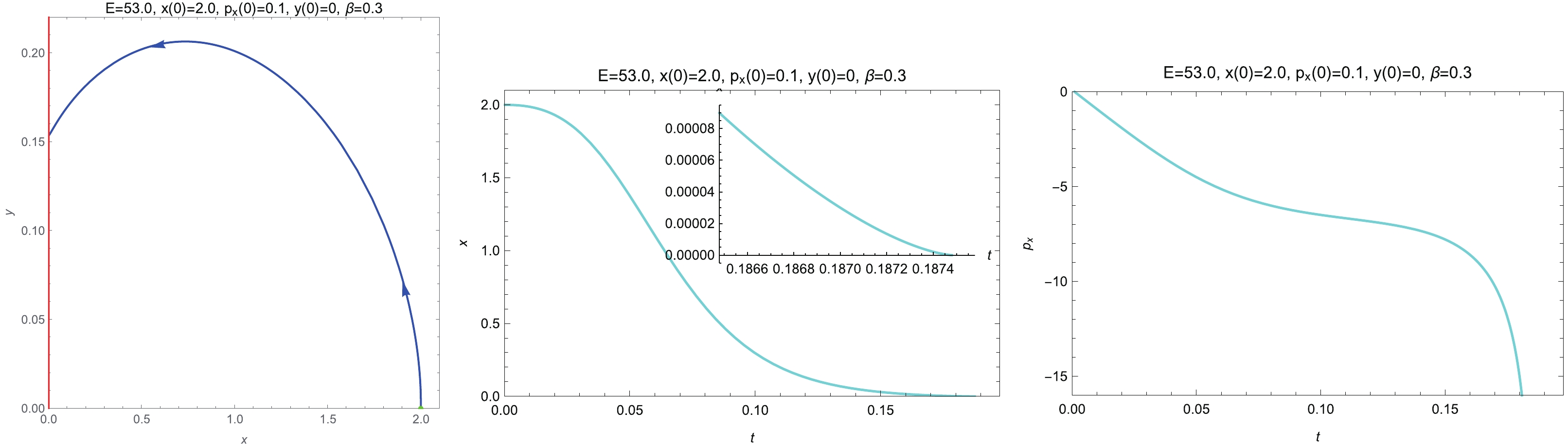
Figure 5. (color online) Plots showing the orbit in the x-y plane,
$ x\left( t\right) $ , and$ p_{x}\left( t\right) $ for$ \beta = 0.3 $ with the initial conditions$ E = 53.0 $ ,$ x\left( 0\right) = 2.0 $ ,$ p_{x}\left( 0\right) = 0.1 $ , and$ y\left( 0\right) = 0 $ . The red line and green dot represent the event horizon and the starting point of the orbit, respectively. The arrows show the increase in simulation time. The inset displays that the particle crosses the horizon at$ t\simeq0.18748 $ . -
LCEs have been proposed to describe the time evolution of perturbations of dynamical systems based on the linearization of equations of motion [73]. For a dynamical system that satisfies the evolution equation
$ {\dot{ x}} = f\left( {{x}}\right) $ , the evolution of the tangent vectors Y along a trajectory$ {{x}}\left( t\right) $ is determined by$ {\dot{ Y}} = {{JY}}, $

(24) where J is the Jacobian matrix, and
$ {{Y}}\left( 0\right) = I $ . The matrix Y characterizes how perturbations of$ {{x}} \left( 0\right) $ propagate to the final point$ {{x}}\left( t\right) $ and defines another matrix$ {{\Lambda}} $ in the infinite time limit,$ {{\Lambda}} = \lim\limits_{t\rightarrow\infty}\frac{1}{2t}\ln\left[ {{Y}}\left( t\right) {{Y}}^{T}\left( t\right) \right] . $

(25) The eigenvalues of
$ {\bf{\Lambda}} $ are defined as LCEs$ \lambda_{i} $ , which measure the exponential expansion rates of infinitesimal perturbations along the trajectory$ {{x}}\left( t\right) $ . The sum of first p largest LCEs can be obtained by computing the expansion rate of a p-dimensional volume along$ {{x}}\left( t\right) $ . In practice, one starts with p linearly independent perturbations, evolves them along$ {{x}}\left( t\right) $ , and performs the QR decomposition [74] (or equivalently, the Gram-Schmidt orthonormalization [75]) at each step to counterbalance all vectors tending to align along the same direction. The expansion rates are then averaged over N successive steps, yielding the LCE spectrum. Here, we employ the method based on the QR decomposition to numerically calculate the LCEs$ \lambda_{i} $ .Among all LCEs
$ \lambda_{i} $ , the maximum Lyapunov characteristic exponent (MLCE)$ \lambda_{\max} $ is of particular interest since a strictly positive MLCE can be considered as an indication of deterministic chaos. The MLCE of the motion of a particle near the horizon of the most general static black hole has recently been argued to satisfy a universal bound [12, 71],$ \lambda_{\max}\leqslant \frac{2\pi T}{\hbar} = \alpha, $

(26) where T is the temperature, and
$ \alpha $ is the surface gravity. The bound$ \left( 26\right) $ was also conjectured to be satisfied for MLCEs of out-of-time-ordered correlators in thermal quantum field theories [76]. Interestingly, it was later shown that the bound$ \left( 26\right) $ can be violated for the motion of a charged massive particle in a charged black hole [77] or when the minimal length effects are taken into account [62].In our case, the dependences of MLCEs on
$ \beta $ are exhibited in Fig. 6 for the initial conditions$ E = 5.0 $ ,$ x\left( 0\right) = 0.9999 $ ,$ y\left( 0\right) = 0 $ , and$ p_{y}\left( 0\right) = 0 $ and$ E = 49.999 $ ,$ x\left( 0\right) = 1.2 $ ,$ y\left( 0\right) = 0 $ , and$ p_{y}\left( 0\right) = 0 $ , respectively. Our numerical results show that MLCEs depend strongly on the choice of the energy E and are quite insensitive to the remaining initial conditions. For$ E = 5.0 $ , we notice that the MLCE is always positive. As$ \beta $ ranges from$ 0 $ to$ 0.006 $ , the MLCE is approximately$ 7\times10^{-4} $ . Interestingly, the MLCE as a function of$ \beta $ has a kink at$ \beta\simeq0.006 $ . When$ \beta\gtrsim0.006 $ ,$ \beta $ becomes significantly greater than zero and grows rapidly as$ \beta $ increases. Since we here choose$ \alpha = 1 $ , the MLCE always satisfies the bound$ \left( 26\right) $ . When$ E = 49.999 $ , the MLCE remains positive as well and has an increasing trend as a function of$ \beta $ , except for several small fluctuations. It is noteworthy that when$ \beta\gtrsim0.02 $ , the bound$ \left( 26\right) $ , which is displayed by the black dashed line in Fig. 6, is violated for the MLCE. As the minimal length corrections in$ {\cal{H}} $ are of the order of$ \beta E^{2} $ , the minimal length effects play a much more important role in the$ E = 49.999 $ case. The observations in Fig. 6 indicate that the minimal length effects tend to make the dynamical system more chaotic, especially when the energy of the system is large.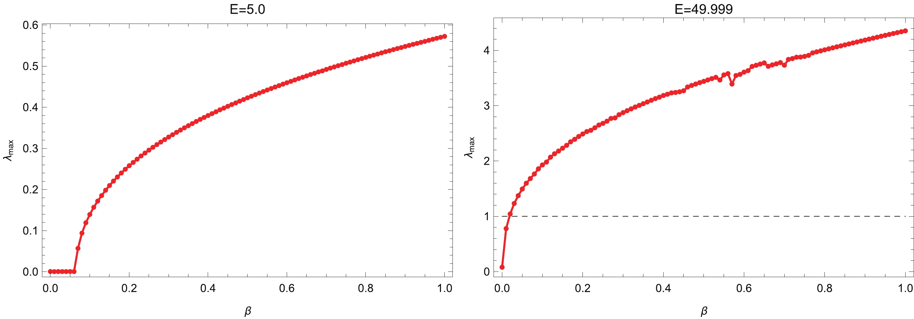
Figure 6. (color online) The maximum Lyapunov characteristic exponents
$ \lambda_{\rm{max}} $ as functions of$ \beta $ for$ E = 5.0 $ (left) and$ 49.999 $ (right). It shows that$ \lambda _{\rm{max}} $ is always positive and primarily increases as$ \beta $ increases, revealing that the minimal length effects could make the trajectories more chaotic. The black dashed line represents the bound$ \left( 26\right) $ . -
Poincaré maps were introduced to map complicated behavior in the phase space to a certain lower-dimensional subspace, called the Poincaré surface of section [78]. Poincaré maps can be used to visualize the dynamics of a chaotic system. In an integrable system, a quasi-periodic orbit fills the Kolmogorov-Arnold-Moser (KAM) torus densely over the course of time, while a periodic (resonant) orbit repeats itself after a few windings. On a Poincaré surface of section intersecting the torus transversally, the crossing points constitute a closed curve and a finite number of fixed points for the quasi-periodic and periodic orbits, respectively. When the integrable system gets perturbed slightly, the KAM theorem [79] states that the quasiperiodic KAM tori are usually deformed but not destroyed, which also leads to KAM closed curves on Poincaré surfaces of section. However, the resonant orbits disintegrate to form Birkhoff chains of islands and thin chaotic layers surrounding the Birkhoff islands of stability on Poincaré surfaces of section [80]. On further deviating from the integrable system, the KAM curves intervening between chaotic layers of different resonances are destroyed, and the chaotic layers can overlap, which generates large scale chaos and stronger chaotic behavior. In short, the observation of a region with scattered points in a Poincaré surface of section is a clear signature of chaos.
Here, we choose the Poincaré surface of section as the one defined by
$ y = 0 $ and$ p_{y}>0 $ , which consequently leaves us a two-dimensional diagram with the vertical$ p_{x} $ axis and the horizontal x axis. Fig. 7 shows the Poincaré surfaces of section for$ E = 5.0 $ with various values of$ \beta $ . We select 22 initial conditions (i.e., E,$ x\left( 0\right) $ ,$ p_{x}\left( 0\right) $ , and$ y\left( 0\right) $ ) and plot the crossing points of the corresponding phase orbits in 8 colors on the Poincaré surfaces of section. The crossing points of the same orbit are in the same color, whereas one color corresponds to$ 2 $ or$ 3 $ orbits. Note that the set of initial conditions of the orbits is the same for each Poincaré surface of section. When$ \beta = 0.1 $ , the Poincaré surface of section consists of KAM closed curves, which shows that the orbits are quasi-periodic. This observation is in agreement with Fig. 2, which also reveals that the orbit with small$ \beta $ is quasi-periodic. However, for a larger$ \beta $ , it displays that the KAM curves start to get destroyed to become scattered plots (e.g., see the lower-right panel in Fig. 7). In short, the growth of the minimal length effects leads to the onset of chaos and a following increase in chaotic behavior of the motion of a particle in the Rindler space.
Figure 7. (color online) The dependence of the Poincaré surfaces of section on
$ \beta $ for the motion of a particle with$ E = 5.0 $ . As$ \beta $ increases, the KAM tori tend to break, which implies that the chaotic behavior becomes stronger.When the energy increases, chaotic regions in Poincaré surfaces of section can be observed for a small value of
$ \beta $ or even$ \beta = 0 $ . We present the dependence of the Poincaré surfaces of section on$ \beta $ with$ E = $ $ 49.999 $ in Fig. 8, which exhibits much richer structures than the$ E = $ $ 5.0 $ case. In fact, chains of islands, chaotic regions with scattered plots, and separatrices in the Poincaré surfaces of section and their evolution with$ \beta $ are seen in Fig. 8, where we plot crossing points of 31 phase orbits in 8 colors. To study the minimal length effects on the chaotic behavior, we focus on the cyan KAM curve on the left side of the$ \beta = 0 $ Poincaré surface of section (upper-left panel of Fig. 8), which is marked by a red arrow and encircled by the chaotic region with scattered brown points. For$ \beta = 0.3 $ , it shows that the cyan KAM curve is not destroyed but gets deformed with a larger width. When$ \beta $ is increased to a value as large as$ 0.5 $ , the lower-left panel of Fig. 8 displays that the cyan KAM curve disintegrates into scattered cyan points so as to form a chaotic region. On further increasing$ \beta $ from$ 0.5 $ to$ 0.7 $ , the chaotic region becomes more dispersed on the Poincaré surface of section, which is shown in the lower-right panel of Fig. 8. These observations lend further support to the conclusion that the minimal length effects can make chaotic behavior of the system stronger.
Figure 8. (color online) The dependence of the Poincaré surfaces of section on
$ \beta $ for the motion of a particle with$ E = 49.999 $ . As$ \beta $ increases from$ 0.1 $ to$ 0.7 $ , the cyan KAM curve marked by a red arrow first gets deformed ($ \beta = 0.3 $ ) and then disintegrates to form a chaotic region ($ \beta = 0.5 $ ), which becomes more dispersed ($ \beta = 0.7 $ ). Thus, as the minimal length effects are increased, the chaotic features become more evident. -
In this paper, we investigated the minimal length effects on the motion of a particle in the Rindler space under a harmonic potential. We first distinguished two different types of trajectories in the motion of the particle. For the first type of trajectories, the particle travels around the fixed point, and the trajectories can be erratic when the minimal length effects are large enough. The particle moving along the second type of trajectories will cross the horizon at a finite Rindler time if the minimal length effects are turned on, whereas it just asymptotically approaches the event horizon in the absence of the minimal length effects. We then exploited Poincaré surfaces of section and LCEs to investigate the chaotic behavior of the system, and as the minimal length effects grew, the following were found:
● Figure 6 showed that, for
$ E = 5.0 $ and$ 49.999 $ , the MLCEs are always positive and generally increase.● Figurre 7 displayed that, for
$ E = 5.0 $ , the KAM curves tend to disintegrate.● Figure 8 exhibited that, for
$ E = 49.999 $ , the cyan KAM curve breaks into a chaotic layer.In light of our numerical results, we come to the conclusion that chaotic behavior is more likely to happen in the presence of the minimal length effects. This is in agreement with earlier observations and generic arguments for a massive particle perturbed away from an unstable equilibrium near the black hole horizon [62], as well as recent findings for the geodesic motion perturbed by the minimal length effects around a Schwarzschild black hole [70]. Specifically, the right panel of Fig. 6 showed that the universal bound of MLCEs
$ \left( 26\right) $ can be violated in the presence of the minimal length effects. Note that the bound$ \left( 26\right) $ was calculated in the framework of general relativity with the absence of quantum gravity effects [12, 71]. The larger the value of MLCEs, the more chaotic the system will be. Therefore, our results further suggest that quantum gravity effects could make classical trajectories in black holes more chaotic.In addition, black hole horizons have been conjectured to be fastest scramblers in nature [81], with the scrambling time
$ t_{s}\sim\hbar T^{-1}\ln S $ , where T and S are the temperature and entropy of the black hole, respectively. Here, we can use Eq.$ \left( 23\right) $ to estimate$ t_{s} $ by relating$ t_{s} $ to the time that it takes to reach the stretched horizon located at$ x = \delta $ , which is roughly one Planck length$ \ell_{\rm p} $ [82, 83]. Then, Eqs.$ \left( 5\right) $ and$ \left( 23\right) $ give$ t_{\rm s}\sim\frac{\hbar}{2\pi T}\left[ \ln\frac{\ell_{\rm p}}{2\pi T}-\frac {3\beta_{0}}{2}\left( \frac{\ell_{\rm p}}{2\pi T}\right) ^{4}\right] , $

(27) where we define a dimensionless parameter
$ \beta_{0}\equiv\beta\ell_{\rm p}^{2} $ . For a Schwarzschild black hole, the scrambling time$ t_{\rm s} $ is$ t_{\rm s}\sim\frac{\hbar}{2\pi T}\left( \ln\frac{16S}{\pi^{2}}-\frac{3\beta _{0}\pi^{4}}{512S^{2}}\right) , $

(28) which indicates that the minimal length effects can make black holes scramble faster. To summarize, in this paper, we proposed a toy model to show that quantum gravity effects tend to increase chaotic behavior and scrambling efficiency of black holes. Further exploration of quantum gravity effects on chaotic dynamics will lend insight into physics of black holes, early universe, and dynamical astronomy.
-
We are grateful to Houwen Wu and Haitang Yang for useful discussions.
-
Consider a scalar field
$ \Phi $ of mass m minimally coupled to a four-vector potential$ A_{a} $ in flat spacetime, governed by the Klein-Gordon equation$\tag{A1} -\left( \partial_{0}-{\rm i}\frac{qA_{0}}{\hbar}\right) ^{2}\Phi+\delta ^{ij}\left( \partial_{i}-{\rm i}\frac{qA_{i}}{\hbar}\right) \left( \partial _{j}-{\rm i}\frac{qA_{j}}{\hbar}\right) \Phi = \frac{m^{2}}{\hbar^{2}}\Phi{,} $

where the index
$ 0 $ denotes the time coordinate, the index$ i = 1,2,3 $ runs over spatial coordinates, and q is the charge of the scalar field$ \Phi $ associated with$ A_{a} $ . For simplicity, we consider an external potential$ A_{a} = \left\{ A_{0},\vec{0}\right\} $ . The Klein-Gordon equation$ \left( A1\right) $ then becomes$\tag{A2} \left[ \left( \partial_{0}-{\rm i}\frac{qA_{0}}{\hbar}\right) ^{2}+\frac{p^{2} }{\hbar^{2}}+\frac{m^{2}}{\hbar^{2}}\right] \Phi = 0, $

where we define the momentum operator
$p_{i}\equiv\dfrac{\hbar}{i}\dfrac{\partial}{\partial x_{i}}$ , and$ p^{2}\equiv\delta^{ij}p_{i}p_{i} $ . In three dimensions, a simple generalization of the deformed algebra$ \left( 1\right) $ reads [34, 37]$ \tag{A3} \begin{aligned}[b] \lbrack X_{i},P_{j}] =& {\rm i}\hbar\left[ (1+\beta P^{2})\delta_{ij}+2\beta P_{i}P_{j}\right] {,}\\ \left[ X_{i},X_{j}\right] =& 0{,} \\ \left[ P_{i},P_{j}\right] =& 0{.} \end{aligned} $

In the pseudo-position representation, one can express
$ X_{i} $ and$ P_{i} $ in terms of the conventional momentum and position operators$ x_{i} $ and$ p_{i} $ ,$ \tag{A4} \begin{aligned}[b] X_{i} =& x_{i},\\ P_{i} =& p_{i}\left( 1+\beta p^{2}\right) , \end{aligned} $

where
$ p_{i} = \dfrac{\hbar}{i}\dfrac{\partial}{\partial x_{i}} $ . Therefore, for the case where the deformed commutation relations$ \left( {\rm A}3\right) $ are considered, the deformed Klein-Gordon equation has been suggested in [84, 85],$\tag{A5} \left[ \left( \partial_{0}-{\rm i}\frac{qA_{0}}{\hbar}\right) ^{2}+\frac{P^{2} }{\hbar^{2}}+\frac{m^{2}}{\hbar^{2}}\right] \Phi = 0, $

where
$ P^{2}\equiv\delta^{ij}P_{i}P_{i}. $ Substituting the ansatz$ \Phi = \exp\left( iS/\hbar\right) $ into Eq.$ \left( {\rm A}5\right) $ and taking the limit$ \hbar\rightarrow 0 $ , one finds that the leading term gives the classical Hamilton-Jacobi equation in deformed spaces,$\tag{A6} \left[ \partial_{0}S-qA_{0}\right] ^{2}-{\cal{X}}\left( 1+\beta {\cal{X}}\right) ^{2} = m^{2}, $

where S is the classical action, and
$ {\cal{X}}\equiv\delta^{ij}\partial_{i}S\partial_{j}S $ .We now generalize the deformed Hamilton-Jacobi equation
$ \left( {\rm A}6\right) $ in flat spacetime to the Rindler space. To this end, we can express the Rindler metric$ \left( 7\right) $ in a local orthonormal frame$ {\rm e}^{a} $ ,$\tag{A7} {\rm d}s^{2} = g_{\mu\nu}{\rm d}x^{\mu}{\rm d}x^{\nu} = \eta_{ab}{\rm e}^{a}{\rm e}^{b}{,} $

where
$ \eta_{ab} $ is the Minkowski metric,$ \mu,\nu \in\left\{ t,x,y,z\right\} $ , and$ a,b\in\left\{ 0,1,2,3\right\} $ . A natural choice for$ {\rm e}^{a} = {\rm e}_{ \mu}^{a}{\rm d}x^{\mu} $ is$\tag{A8}\begin{aligned}[b]& { e}^{0} = \alpha x{\rm d}t,\;\;\;\;\;{ e}^{1} = {\rm d}x,\\&{ e}^{2} = {\rm d}y,\;\;\;\;\;{ e}^{3} = {\rm d}z, \end{aligned}$

which gives the vierbein fields
$ { e}_{ a}^{\mu} $ $\tag{A9} { e}_a^\mu = \left( {\begin{array}{*{20}{c}} {{{\left( {\alpha x} \right)}^{ - 1}}}&0&0&0\\ 0&1&0&0\\ 0&0&1&0\\ 0&0&0&1 \end{array}} \right). $

Since the local orthonormal frame corresponds to locally inertial coordinates, the deformed Hamilton-Jacobi equation in the local orthonormal frame is simply given by the deformed Hamilton-Jacobi equation in flat space, namely Eq.
$ \left( {\rm A}6\right) $ . In contrast, the vierbein fields$ { e}_{ a}^{\mu} $ enable conversion between spacetime and local Lorentz indices,$\tag{A10} \begin{aligned}[b]\partial_{0}S-qA_{0} =& e_{ 0}^{\mu}\left( \partial_{\mu}S-qA_{\mu }\right) = \left( \alpha x\right) ^{-1}\left( \partial_{t}S-qA_{t}\right) {, }\\\partial_{1}S =& \partial_{x}S{, }\partial_{2}S = \partial _{y}S{, }\partial_{3}S = \partial_{z}S.\end{aligned} $

Plugging Eq.
$ \left( {\rm A}10\right) $ into Eq.$ \left( {\rm A}6\right) $ , we can express the deformed Hamilton-Jacobi equation in the Rindler coordinates,$\tag{A11} \frac{1}{\alpha^{2}x^{2}}\left[ \frac{\partial S}{\partial t}-qA_{t}\right] ^{2}-{\cal{X}}\left( 1+\beta{\cal{X}}\right) ^{2} = m^{2}, $

where S is the classical action, and
$ {\cal{X}} \equiv\left( \partial_{x}S\right) ^{2}+ \left( \partial_{y}S\right) ^{2}+\left( \partial_{z}S\right) ^{2} $ . For the four-vector potential$ A_{\mu} = \left\{ A_{t},\vec{0}\right\} $ , the potential energy V of the scalar is①$\tag{A12} V = -qA_{t}{.} $

Hence, Eqs.
$ \left( {\rm A}11\right) $ and$ \left( {\rm A}12\right) $ lead to the deformed Hamilton-Jacobi equation$ \left( 12\right) $ with the potential V in the Rindler coordinates.
Minimal length effects on motion of a particle in Rindler space
- Received Date: 2020-08-23
- Available Online: 2021-02-15
Abstract: Various quantum theories of gravity predict the existence of a minimal measurable length. In this paper, we study effects of the minimal length on the motion of a particle in the Rindler space under a harmonic potential. This toy model captures key features of particle dynamics near a black hole horizon and allows us to make three observations. First, we find that chaotic behavior becomes stronger with increases in minimal length effects, leading predominantly to growth in the maximum Lyapunov characteristic exponents, while the KAM curves on Poincaré surfaces of a section tend to disintegrate into chaotic layers. Second, in the presence of the minimal length effects, it can take a finite amount of Rindler time for a particle to cross the Rindler horizon, which implies a shorter scrambling time of black holes. Finally, the model shows that some Lyapunov characteristic exponents can be greater than the surface gravity of the horizon, violating the recently conjectured universal upper bound. In short, our results reveal that quantum gravity effects may make black holes prone to more chaos and faster scrambling.


 DownLoad: